Introduction
This document is meant to help new robotics users and specifically users of the Pheeno robotic platform get used to onboard sensing typically used as feedback in control theory. Typically when learning the theory behind controllers the feedback term is assumed to be perfect and known. In reality, these feedbacks are based on sensor measurements that must be calibrated properly with limitations that should be known. There are many different types of sensors with large ranges of precision and cost. Here, the focus will be put on the sensors onboard the Pheeno platform and fusing their measurements to produce reliable feedback.
Getting to Know the Onboard Sensors will provide a high level introduction to the sensors on board the Pheeno robotic platform, their strengths and weaknesses, and how they should be used. The Calibration section will go into how and why to calibrate sensors on board the robot. The Sensor Fusion for State Feedback section will introduce different methods to combine sensor measurements into reliable, robust position and orientation estimates for the robot. It will also briefly go into the pros and cons of each fusion.
Getting to Know the Onboard Sensors
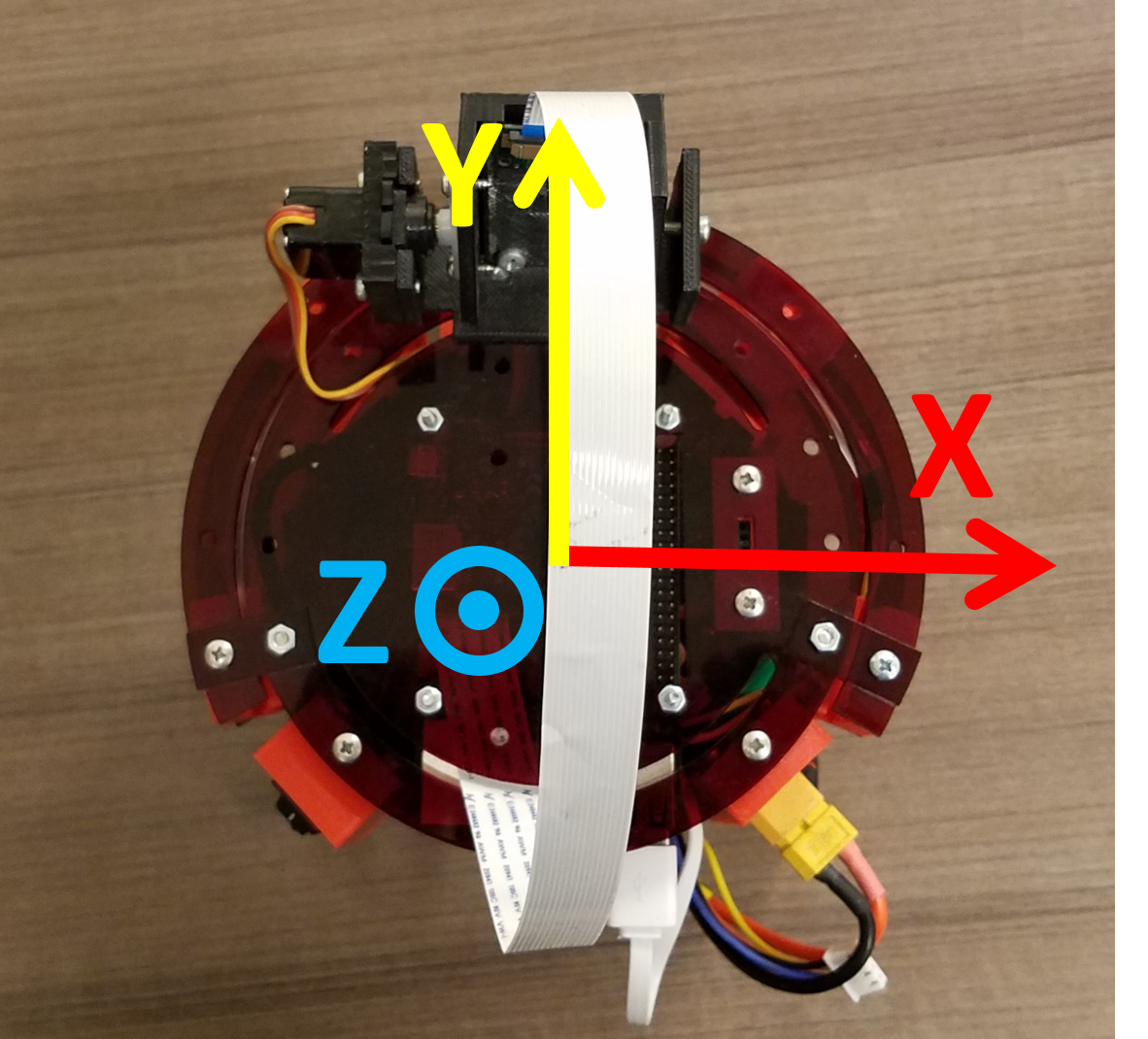
Pheeno is equipped with a MiniIMU-9 v5 made by Pololu. This little board contains a 3-axis accelerometer, 3-axis gyroscope, and 3-axis magnetometer. Figure 1 shows the ideal reference frame of the MiniIMU-9 v5 aligned with Pheeno’s reference frame. Pheeno is also equipped with 6 infrared (IR) distance sensors, a quadrature encoder on each motor, and an RGB camera. Each of these sensors alone are very powerful, however, they each have critical weaknesses which will be explored below. Together, with the help of a little mathematics, these sensors make up for each other’s weakness and allow Pheeno to figure out where it is in space and what its surroundings are like.
One thing that will not be covered in this document is converting raw data/voltages provided by the MinIMU-9 v5 or any of the sensors on the robot. For reference, sensors typically output analog or digital voltages which must be converted to digital signals that may then be transformed to standard units by a micro processor. Other, more complex sensors, have micro chips on board that use communication protocols like Inter Integrated Circuit Communications, $I^2 C$, and Serial Peripheral interface (SPI).
A typical inertial measuring unit (IMU) like the MiniIMU-9 v5 will not output raw data in any units that are useful to the operator. IMUs like this typically have different operating ranges that can be set by the user. For whatever range is chosen by the user, a conversion factor is typically given in the datasheet associated with the IMU. It is important to note however, all sensors on a robot are quantized at some resolution (meaning whatever continuous source they measure will be represented at discrete increments). Typically there is a trade off between the resolution of measurements and the range of values that can be measured. For example, the standard setting for the gyroscope on Pheeno is set to measure an angular rotation rate range of $\pm 245 ^\circ/s$. This allows for a measurement resolution of $0.00875^\circ/s$. This is fine for determining rotations on a small robotic platform like Pheeno but this concept should not be ignored. The resolution and range of any sensor on board should be chosen as appropriate to the application.
Accelerometer
An accelerometer measures its linear acceleration along several principle directions. In Pheeno’s case the MiniIMU-9 v5 has a 3-axis accelerometer allowing the user to know how the robot’s linear acceleration in all three possible dimensions. From this sensor alone the user can infer the direction the robot is accelerating as well as its pitch and roll angle (if you are unfamiliar with roll and pitch angles, refer to Figure 12, they will be further explained later). If Pheeno drives off a cliff, it will be very apparent from the accelerometer’s sensor measurements that it is tumbling to its doom.
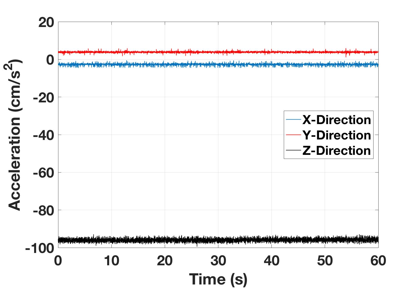
To explain what an accelerometer should be used for, raw accelerometer data from a resting and rotating Pheeno will be analyzed. First, Pheeno was placed onto a table top and 60 seconds of accelerometer data was recored at a rate of 100 Hz (every 10 ms). Figure 2 shows the raw time series data of the the acceleration felt along each axis of the accelerometer. This data shows the readings are noisy but very stable. The accelerometer is currently just measuring gravity which should be only in the z-direction. However, from this plot we can see there are slight measurements in the x and y direction as well. This is due to slight misalignment between the IMU board orientation and Pheeno’s resting orientation caused during manufacturing of the robot. A misalignment similar to this should be present in every robot. From this data, it is possible to calibrate the accelerometer and determine how tilted the board is relative to the robot, thus aligning their reference frames.
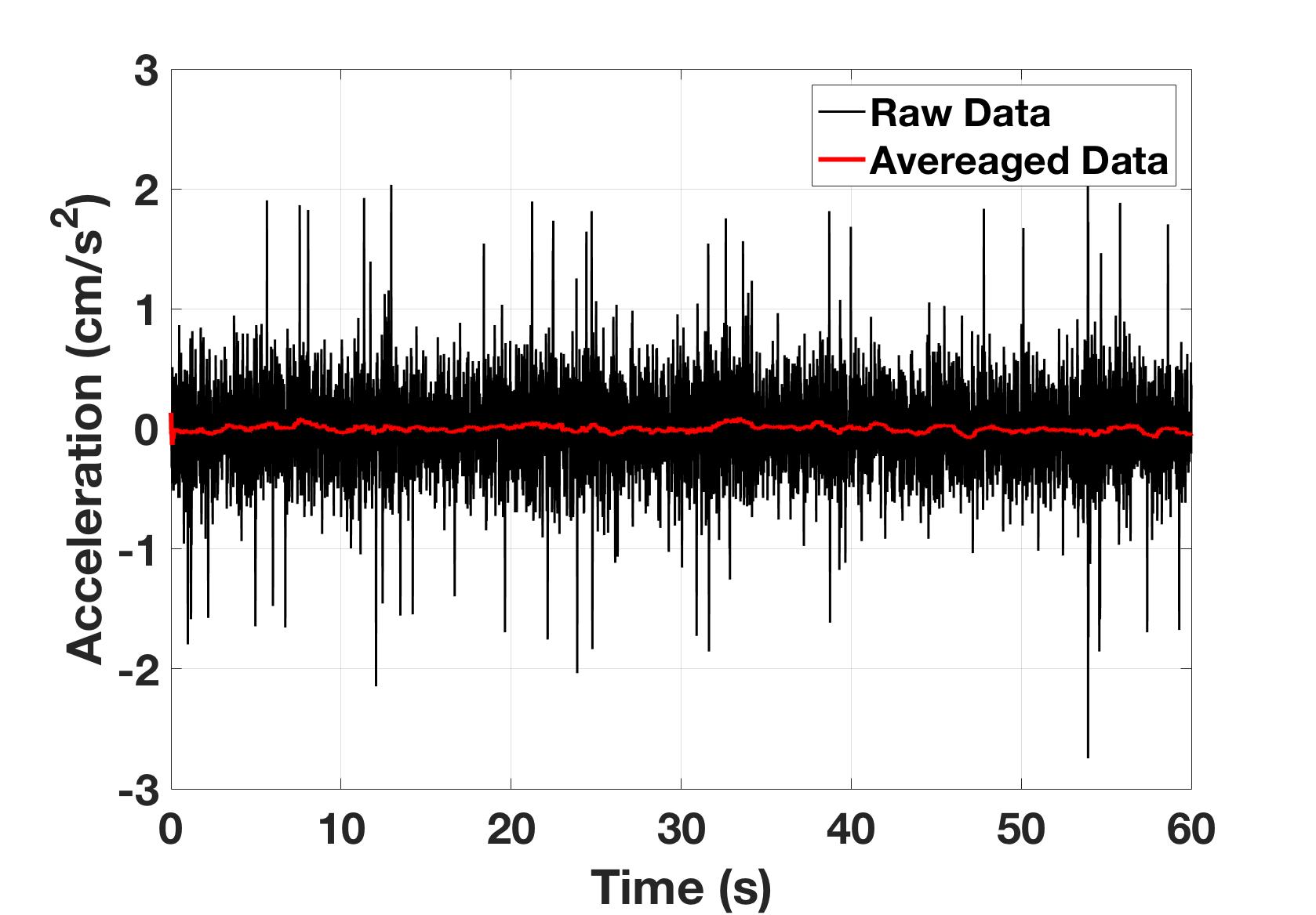
Figure 3 shows the acceleration along the Y-Direction of the accelerometer after the time averaged bias has been subtracted. From this we can see most of the noise in the raw sensor measurements (black line) is around $\pm 1 cm/s$. If the sensor is moved around quickly, the accelerations of the motion will be measured and the vibrations during the motion will amplify the noise. It should be noted how the $100$ sample running mean of the signal (red line) provides a much more stable signal. This shows the noise content of the signal is at a high frequency and a low pass filter can be used to get reliable measurements from the accelerometer. However, a low pass filter will not track quick acceleration changes well by its design. This will be addressed later.
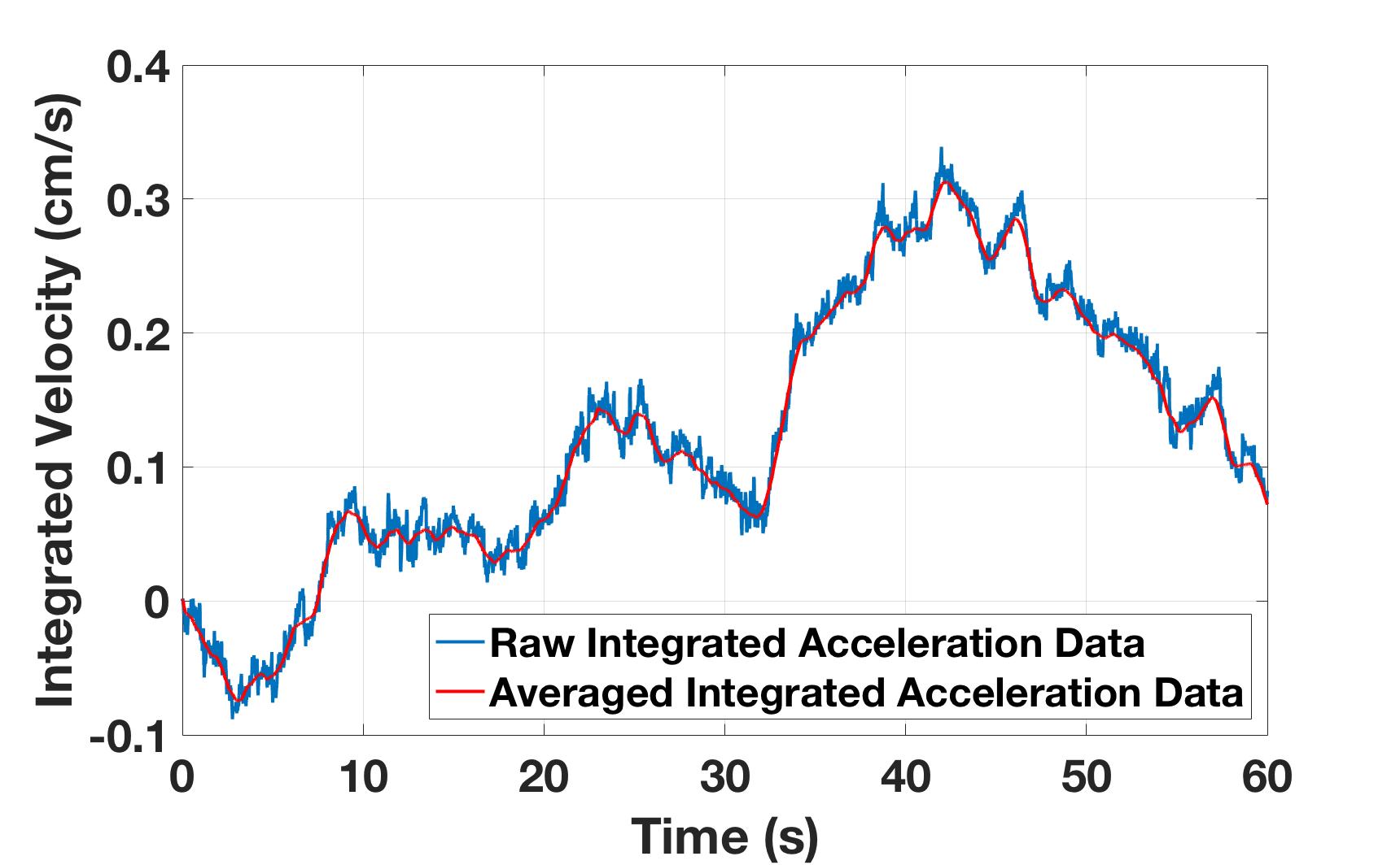
Figure 4 shows the velocity approximated from the accelerometer if the accelerometer measurements are integrated. Over small time intervals this works reasonably well but over long time periods integration error overwhelms the approximation. Recall, this is from an accelerometer at rest on a table. During the $60$ second interval pictured, the at rest accelerometer yields non zero velocities. Note this happens even when the signal is averaged and the noise is not as severe.
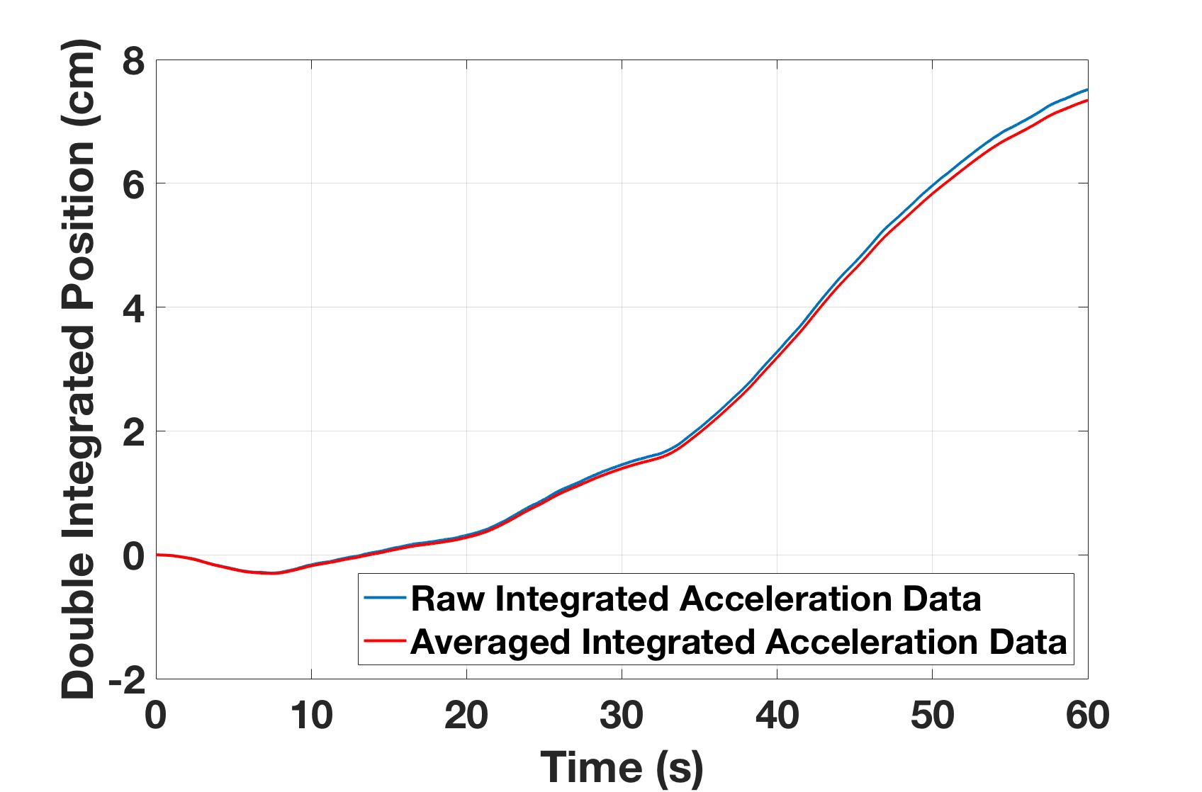
Figure 5 shows the position approximated from integrating the accelerometer measurements twice. As expected this leads to compounded integration error which causes this position approximation to be $7.5$ cm from its original location in $60$ seconds. If left to rest for a longer period of time, the accelerometer’s estimation of position will only get worse.
From these results, an accelerometer should really only be used to determine the angle of orientation of the robot (pitch and roll), the acceleration of the robots motion, and sometimes the velocity of the robot over short time periods. These become tricky when the robot is actually being driven around since acceleration from the motion of the robot and interaction between the robot and its environment is measured by the accelerometer. If the robot is in a terrain where the ground changes the orientation of the robot drastically this challenge becomes even more difficult but not impossible. Later the accelerometer’s readings will be combined with other on-board sensors to give an accurate measurement of the robot’s orientation and linear acceleration. An accelerometer should almost never (really never) be used to approximate the robot’s position through integration, especially over longer time scales. Integration error adds up very quickly and throws off a robot’s localization significantly.
Gyroscope
Gyroscopes measure the rotational velocity about several principle axes. In Pheeno’s case, the MiniIMU-9 v5 has a 3-axis gyroscope allowing the user to know how fast the robot is rotating about each axis. This sensor is typically used in parallel with the magnetometer and accelerometer to determine the angular orientation of the robot at all times. Unlike the accelerometer and magnetometer which typically have very accurate but noisy signals that cannot detect fast motions, gyroscopes are great at capturing fast rotations without being affected by the accelerations, but their orientation estimates will drift over time due to integration error.
To better understand a gyroscope’s output and limitations Pheeno was manually rotated $90$ degrees [$\sim 1.57$ radians] back and forth about its z-axis for $60$ seconds. The raw data is shown in Figure 6(a). Due to the misalignment of the MiniIMU-9 v5 board with the robot’s reference frame, there is noticeable rotation about the z-axis (yaw) and y-axis (roll) and x-axis (pitch). This can be corrected in calibration which will be discussed in the Gyro Calibration section. The corrected data are shown in Figure 6(b). This data shows that the gyroscope is very good at capturing consistent angular rate data at high frequencies with a relatively small amount of noise. Figure 7(a) shows the data from Figure 6(a) integrated once to determine the Pheeno’s orientation. Again, this data is uncalibrated and the errors from the misalignment and offset add up quickly. After calibration this runaway integration decreases as shown in Figure 7(b). The yaw orientation estimate is fairly consistent showing approximately $90$ degrees of rotation back and forth at two different rates. Due to the nature of the rotation (manually turning the robot back and forth and eyeballing a $90 ^{\circ}$ rotation) there is slight deviation in the periods of the rotations as well as the magnitudes. The calibration here is not perfect as some of the rotation is captured in the roll estimate but this is small and with more exact and thorough calibration can be suppressed further.
The weakness of gyroscope measurements is commonly referred to as drift, where the integration error causes the estimate to “drift” in one direction. Figure 7(b) shows this as the yaw estimate is slowly becoming more and more negative. Gyroscopes are great at estimating rotations over small time scales but suffer if this estimate is done for long periods of time. While frustrating, it is important to note this is the opposite of the accelerometer measurements which are not reliable over short time spans but very reliable over long ones because their orientation estimate does not rely on integration and thus will not drift. However, accelerometers are only able to recover two angles of orientation, which have been chosen to be pitch (rotation about the x-axis) and roll (rotation about the y-axis). In order to determine the robots yaw angle (rotation about the z-axis) for long time spans, the robot requires an additional sensor, the magnetometer.
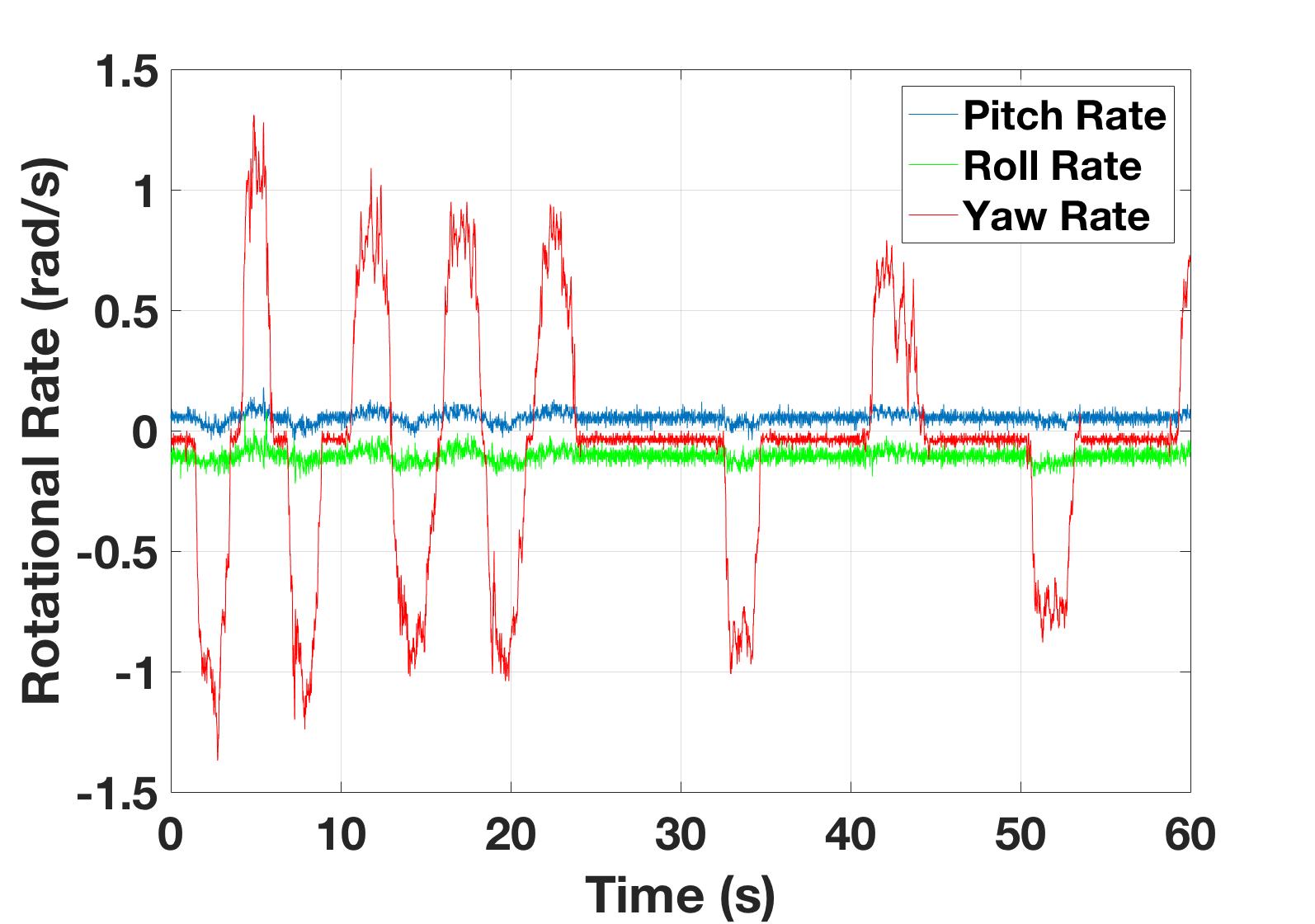
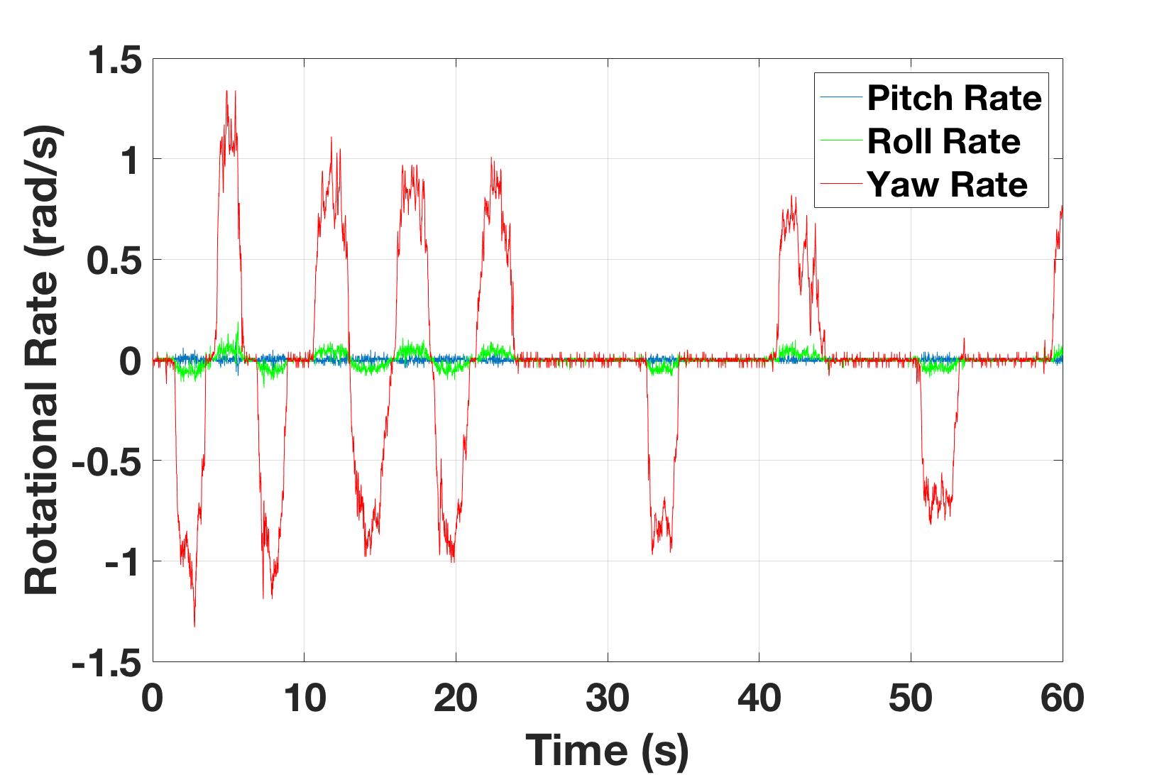
Figure 6: The time evolution of the (a) uncalibrated and (b) calibrated rotational velocity measurements about each axis measured by the gyroscope on board Pheeno. The robot was rotated $90$ degrees back and forth over a $60$ second period.
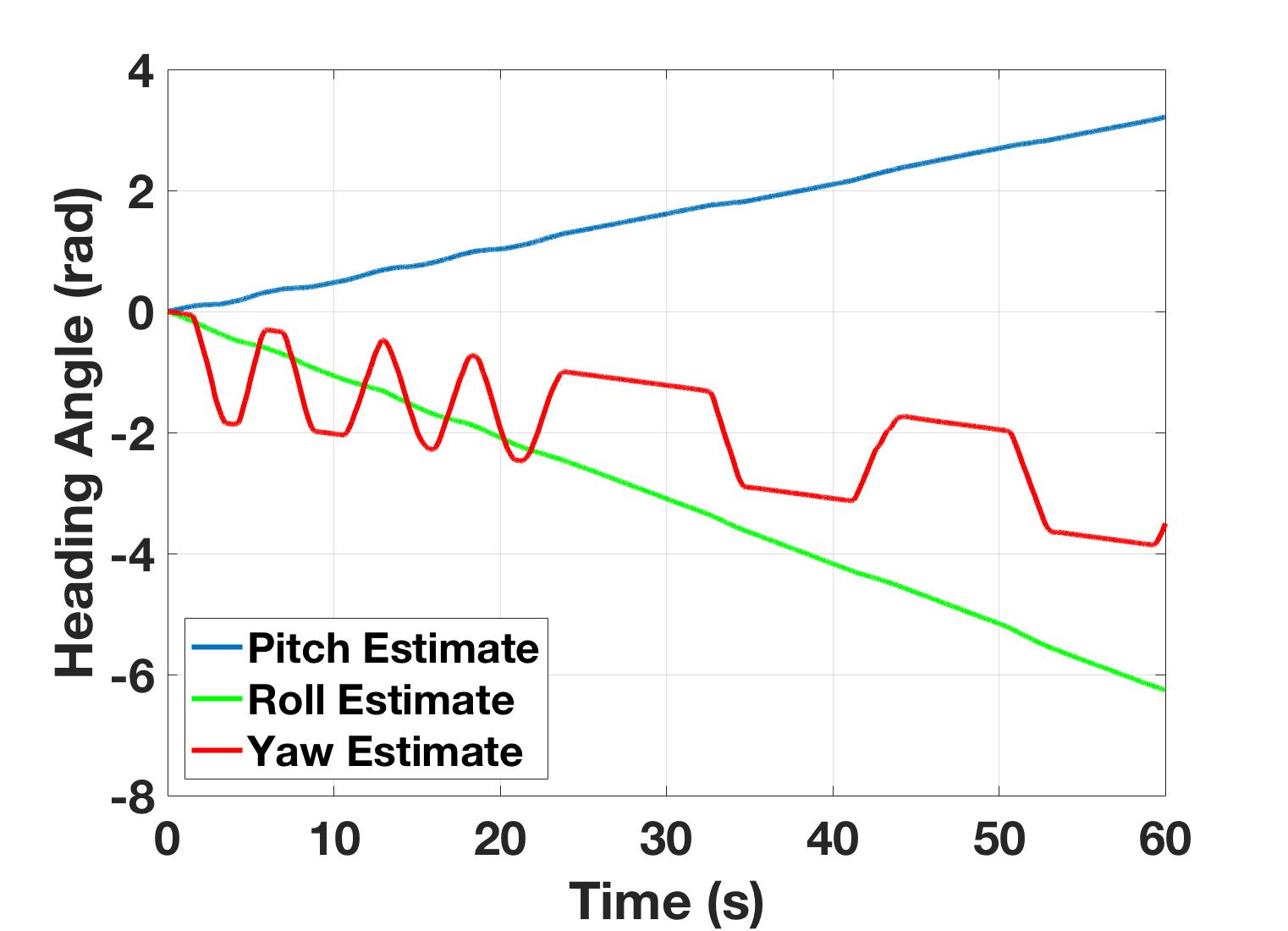
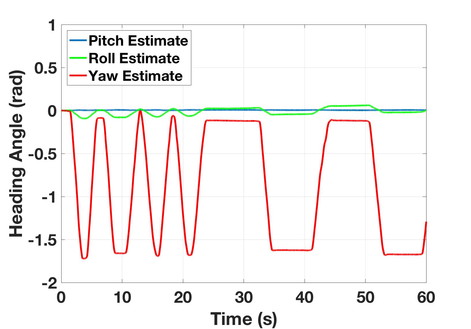
Figure 7: The time evolution of Pheeno’s estimation of orientation from integration of (a) uncalibrated and (b) calibrated gyroscopic rate measurements in Figure 6(a) and Figure 6(b). The robot was rotated $90$ degrees back and forth over a $60$ second period.
Magnetometer
The magnetometer is very similar to an accelerometer. However, in stead of measuring a gravity vector it measures the direction of the magnetic field surrounding it. The magnetometer on the MiniIMU-9 v5 represents the magnetic field vector along the same axis as the accelerometer. Its readings do not drift (given there are no magnetic anomalies) but are noisy like the accelerometer.
Typically the magnetic field being read is dominated by the earth’s magnetic field. This field can easily be influenced by other magnetic sources like wires carrying large currents in buildings, large motors onboard the robot, and large metal beams in buildings. Luckily Pheeno is a small robot that uses low current micro metal gear motors that do not produce large enough magnetic fields to really influence the magnetometer readings. In larger robots with bigger motors, the magnetometer’s proximity to the motors should be accounted for. Since Pheeno is typically used indoors, it is important for the user to determine if the room the robot is being used in has a consistent magnetic field. If the field changes too drastically in some areas those areas must be avoided or the magnetometer cannot be used reliably.
Assuming the area the robot is in has a consistent magnetic field, when the robot is rotated the measured magnetic field vector should point to the surface of a sphere centered at the origin with radius equal the strength of the present magnetic field. However, without calibration the readings from a rotating robot will look like Figure 13(a). This plot is 2D planar slices of the 3D ellipsoid showing the resulting measurements are not a sphere centered at the origin. Typically the offset of this ellipsoid from the origin is referred to as hard iron error and the directional scaling in each direction is called soft iron error. It is crucial the magnetometer is calibrated properly to correct both these errors. If the magnetometer is not calibrated correctly, Pheeno will be unable to reliably determine its yaw angle and thus heading angle. This will be further discussed in the Magnetometer Calibration section.
Motor Encoders
Motor encoders are used to count the number of shaft rotations that have occurred. Figure 8 is a cartoon of a simple optical encoder. The wheel that is attached to the shaft blocks the light from hitting the sensor at set increments which creates a signal that is able to be measured by a micro controller. This is the foundation of all encoders. An emitter’s signal (the light source in this case) is interrupted by a shaft attachment creating known patterns (e.g. 12 per rotation, a known pattern at a set angle, etc). However, there are many variations of encoders which use different emitters (e.g. magnetic, optical, electrical contact, resistance, etc.), have different number of sensors, and should be used in different scenarios.
Encoders typically fall into two classes, incremental and absolute. Incremental encoders, shown in the top of Figure 8, are only able to determine whether a rotation of the shaft has taken place and increment or decrement their rotation count. Absolute encoders, shown in the bottom of Figure 8, are able to determine the orientation of the shaft at any time (within some angular resolution) due to a specific feedback at each orientation. Typically incremental encoders are less expensive than absolute encoders but are susceptible to errors if counts are missed due to power loss or other factors. This can be a catastrophic problem in a robotic arm assembling a car frame but is less consequential in a small robotic platform like Pheeno.
Mobile platforms like Pheeno use encoders to count the number of rotations each wheel has made. This can then be used as feedback to determine how fast the motor is actually rotating the platforms wheels and how far the robot’s body has traveled or rotated. However, this position and orientation estimates are extremely vulnerable to non level surfaces and wheel slip. Both of these problems cannot be remedied by absolute encoders and thus Pheeno uses incremental encoders, specifically quadrature encoders.
Unlike standard (one sensor) encoders, which can only determine speed and displacement, quadrature encoders can determine velocity and direction. The major difference here is quadrature encoders can determine the direction of rotation of a shaft. It is possible to use a normal encoder on a motor and trust the encoder is rotating in the direction commanded, however, it is a horrible idea to assume your input direction translates to your output direction. In a small robot like Pheeno if the motors are turned off and allowed to rotate passively, this rotation will be captured correctly by quadrature encoders and will not necessarily be captured correctly by normal encoders.
Pheeno uses magnetic quadrature encoders that use hall effect sensors to detect rotational motion of its motors. Hall effect sensors are used because the emitter and sensor do not need to be well aligned and are not effected by lighting conditions like optical encoders. The encoder is mounted on an extended back shaft of a micro metal gear motor which rotates at the speed of the motor before the rotation is geared down to the wheel shaft. This allows for higher resolution measurement of the wheel rotation.
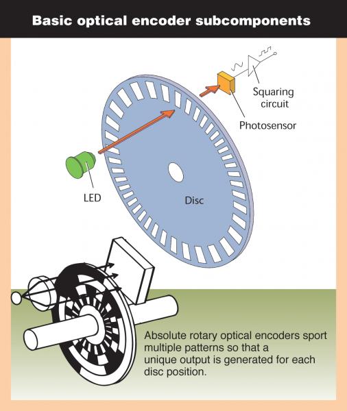
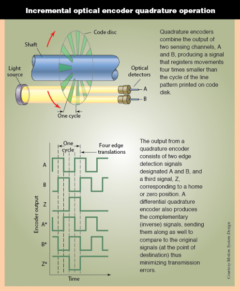
Figure 8: Encoder diagrams. Figure from [1].
Infrared Distance Sensors
Pheeno uses six Sharp GP2Y0A41SK0F analog infrared distance sensors to sense linear distance of objects around the robot. These sensors were chosen due to their price instead of an expensive Light Detection And Ranging (LIDAR), sometimes referred to as Light Imaging, Detection, And Ranging, sensors. They also do not have issues with ghost echoes like Sound Navigation And Ranging (SONAR) sensors. Five are uniformly distributed radially along the front $180^\circ$ of the robot with one in the rear. These are made to measure $4$ cm to $30$ cm distances in front of the sensor. However, they can be exchanged with any other IR sensor with JST mounts for different distance ranges (given the power, signal, and ground connections are the same).
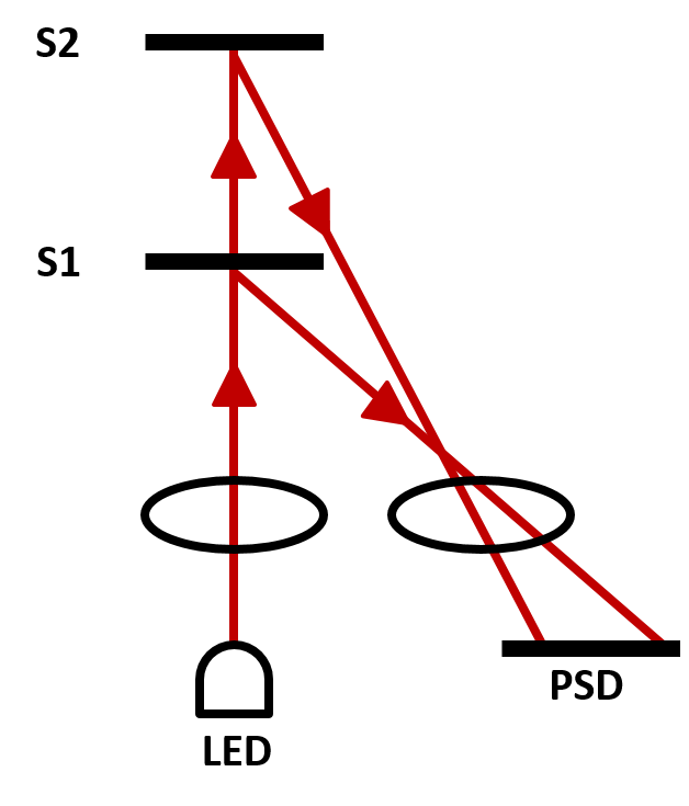
Figure 9 shows a cartoon representation of how a Sharp IR distance sensor works. A light emitting diode (LED) emits a beam of light through a lens which reflects off a surface and hits a different location on the position-sensible photo detector (PSD). Based on the location struck by the reflected beam, a distance measurement can be produced. This method of measuring distance has a few drawbacks that should be recognized. The first is, small or very curved surfaces (e.g. a chair leg) can not always be observed by the IR sensor because the initial beam will miss the object or the reflection will miss the PSD. The second reason is, light absorbing surfaces (e.g. darker surfaces) will absorb a lot of the sensing beam and thus will not cause a reflected beam. The final is a common problem in most light based distance sensors. The beam is very thin and thus the sensor must be aligned both in height and orientation with the object to create a reliable measurement.
Camera
Pheeno has an optional Raspberry Pi Camera attached to the top of the robot which allows visual information to be captured, processed, and/or transmitted to other devices. This camera is a five megapixel fixed-focus camera that is able to capture $1080p$ resolution at $30$ frames per second (FPS), $720p$ resolution at $60$ FPS, or lower resolutions at $90$ FPS. These frame rates are possible in theory but in naive practice these frame rates drop due to the robot’s processing capabilities (on board the Raspberry Pi). When performing further processing on the robot, these frame rates drop even further unless more advanced techniques beyond the scope of this document are implemented.
Calibration
This section will go through the calibration required to use Pheeno’s on-board sensor suite correctly. This is meant as a high level calibration, meaning the misalignment of the sensors and their sensing ranges will be corrected. Typically these sensors should be calibrated to deal with temperature changes and other factors but that will not be covered.
Without calibration the on-board sensors could still be used but would yield information with systematic errors constantly. Calibration really only needs to be done to the IMU. The accelerometer calibration will be covered in the Accelerometer Calibration section, gyroscope calibration will be shown in the Gyro Calibration section, and the magnetometer calibration will be done in the Magnetometer Calibration section. Encoders typically work out of the box. Any calibration needed to detect the changes in magnetic or optical field created by the encoder has already been done before purchasing the sensor. Due to this, the Encoder Calibration will discuss common problems that can be avoided with counting incremental encoders and how to transform counts to linear distances traveled by the wheels of the robot. IR distance sensors typically have a conversion factor available in the data sheet that transforms the voltage read to distance, however, it is a good idea to not blindly trusting data sheets and fit distance data to readings on their own. Cameras, like the one on Pheeno, are typically plug and play. However, it should be noted there are auto calibration functions constantly going on in the background of these web-cam like cameras which are actively focusing the picture, letting in an ample amount of light, and auto-balancing the colors. There are ways to do this manually but that will not be covered here.
Accelerometer Calibration
The data from the accelerometer at rest in the Accelerometer section suggested the orientation of the IMU was not the same as the robot due to manufacturing errors. If this slight misalignment was ignored, the accelerometer would pass biased acceleration information to the robot every measurement. This would cause errors in the orientation calculations as well as acceleration measurements of the robot. A typical mistake made by new robotic users is to simply subtract off this bias measured when the robot is at rest. This does not solve the problem as any acceleration will not be measured in the same reference frame as the robot’s. Even worse, because the gyroscope measures rotational velocity and the magnetometer measures the magnetic field about the same axes, the angular rotation and magnetic field measurements would be in the wrong reference frame as well.
To correct this, the same resting accelerometer data from the Accelerometer section will be used. First, the bias in the data must be identified. Here, it is assumed the sensor has additive white Gaussian noise (AWGN). This assumption means any noise in the sensor is uniform across frequencies, can be described by a Gaussian (normal) distribution, and is added to the true signal. To back up this assumption, the resting accelerometer signal in the x-direction from the Accelerometer section is analyzed. Figure 10 shows the single-sided amplitude spectrum of the resting accelerometer data along the x-axis after a fast Fourier transform. This shows the expected spike at zero because the measurement is just a static signal as well as spikes along the rest of the frequencies from noise. This supports the white noise assumption as there are no significant peaks besides the signal. Figure 11 displays the histogram of the measurements along the x-axis from the accelerometer at rest. While there is a small bump on the left tail of the distribution, this still supports the Gaussian noise assumption.
From the AWGN assumption, the bias in each direction is the average acceleration along each axis. This bias vector allows the user to identify the roll and pitch angle differences between the reference frame of the IMU and the resting Pheeno’s reference frame. Figure 12 is a cartoon representation of Pheeno in orientations that would create a roll, pitch, and yaw angles. From our single at rest accelerometer measurement it is impossible to calibrate all three angles. Any gravity measurement will wind up on a unit gravity sphere which only requires two angle parameters to describe fully. Another way to think about this is if the z-axis of the robot’s reference frame and the IMU’s reference frame were aligned, any yaw rotation would cause the same measurement of $1g$ along the z-axis. However from this it is still possible to calibrate the roll and pitch offset between the IMU and the robot reference frames.
With a bit more mathematical rigor, Pheeno’s IMU oriented in Earth’s gravitational field $\vec{g}$ undergoing a linear acceleration $\vec{a_e}$ in the earth’s reference frame will produce a reading $\vec{M}$ of,
where $\textbf{R}$ is the rotation matrix that relates the IMU’s reference frame to the Earth’s. Since we are dealing with orientation data where the robot is at rest on a surface parallel to the Earth’s surface, the z-axis of the robot’s reference frame is aligned with the z-axis of the reference frame of the Earth, this equation simplifies to,
The rotation matrices that describe the roll, pitch, and yaw rotations shown in Figure 12 are described as,
Using these rotation matrices there are six unique rotation orders that can be done to produce the same rotation; $\boldsymbol{R_y}(\phi)\boldsymbol{R_x}(\theta)\boldsymbol{R_z}(\psi)$ (Roll, Pitch, Yaw), $\boldsymbol{R_y}(\phi)\boldsymbol{R_z}(\psi)\boldsymbol{R_x}(\theta)$ (Roll, Yaw, Pitch), $\boldsymbol{R_x}(\theta)\boldsymbol{R_y}(\phi)\boldsymbol{R_z}(\psi)$ (Pitch, Roll, Yaw), $\boldsymbol{R_x}(\theta)\boldsymbol{R_z}(\psi)\boldsymbol{R_y}(\phi)$ (Pitch, Yaw, Roll), $\boldsymbol{R_z}(\psi)\boldsymbol{R_x}(\theta)\boldsymbol{R_y}(\phi)$ (Yaw, Pitch, Roll), $\boldsymbol{R_z}(\psi)\boldsymbol{R_y}(\phi)\boldsymbol{R_x}(\theta)$ (Yaw, Roll, Pitch). These rotation orders are not commutative, like most matrix multiplications, and multiplying them out yields different matrices. To solve for roll and pitch, expanding the pitch, roll, yaw matrix multiplication yields,
Using this matrix in Equation 1 with $\vec{g} = [0 \hspace{0.1cm} 0 \hspace{0.1cm} -1]^T$ yields,
which is only dependent on the pitch, $\theta$, and roll, $\phi$, angles. Using the average measurement vector, it is possible to solve Equation 2. It should be noted that the vector on the right side of Equation 2 always has a length of $1$, thus $\vec{M} = [M_x \hspace{0.1cm} M_y \hspace{0.1cm} M_z]^T$ should be normalized. Solving Equation 2 for the pitch and roll angles yields,
Note that the pitch angle has two negatives that could be canceled. These are left in purposefully so that when solving for the angle and using and atan2() function the user does not get the wrong angle.
Now to determine the yaw angle offset, Pheeno is pitched at a known angle like in Figure 12(b). The new measured gravity vector should now be $g = [0 \hspace{0.1cm} -\sin(\theta_d) \hspace{0.1cm} -\cos(\theta_d)]$ where $\theta_d$ is the known inclination of the robot. Substituting this into Equation 1 yields,
where $M_p$ is the accelerometer measurement vector when Pheeno is pitched at angle $\theta_p$. In this equation there is no $\boldsymbol{R_z}(\psi_{xyz})$. This is because previously $\psi_{xyz}$ was not able to be solved for. Thus, it can be chosen arbitrarily. If chosen to be $\psi_{xyz} = 0$, $\boldsymbol{R_z}(\psi_{xyz})$ is a 3x3 identity matrix. To simplify this equation, substitute,
This allows for an explicit solution for $\psi$,
The rotation matrix which aligns the IMU’s reference frame with Pheeno’s is then,
These angles should be saved. To use this calibration properly, any measurement should be rotated through this matrix.
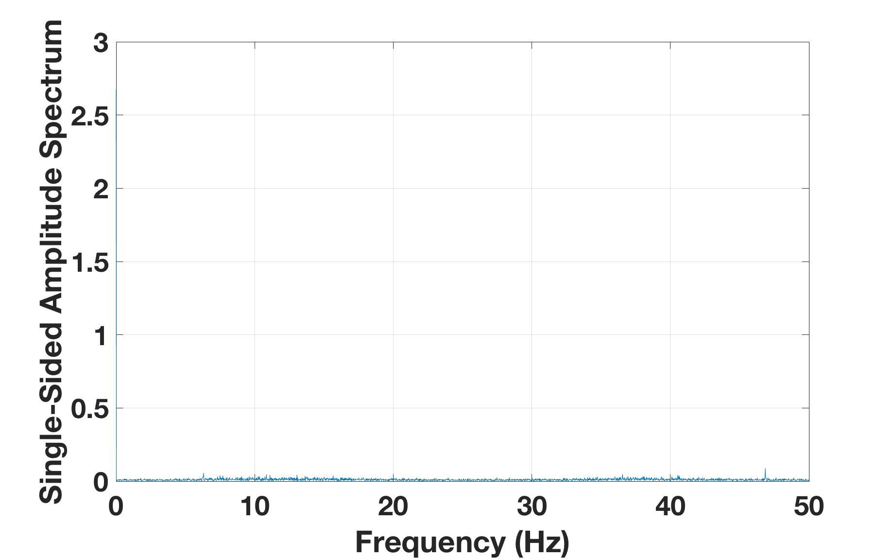
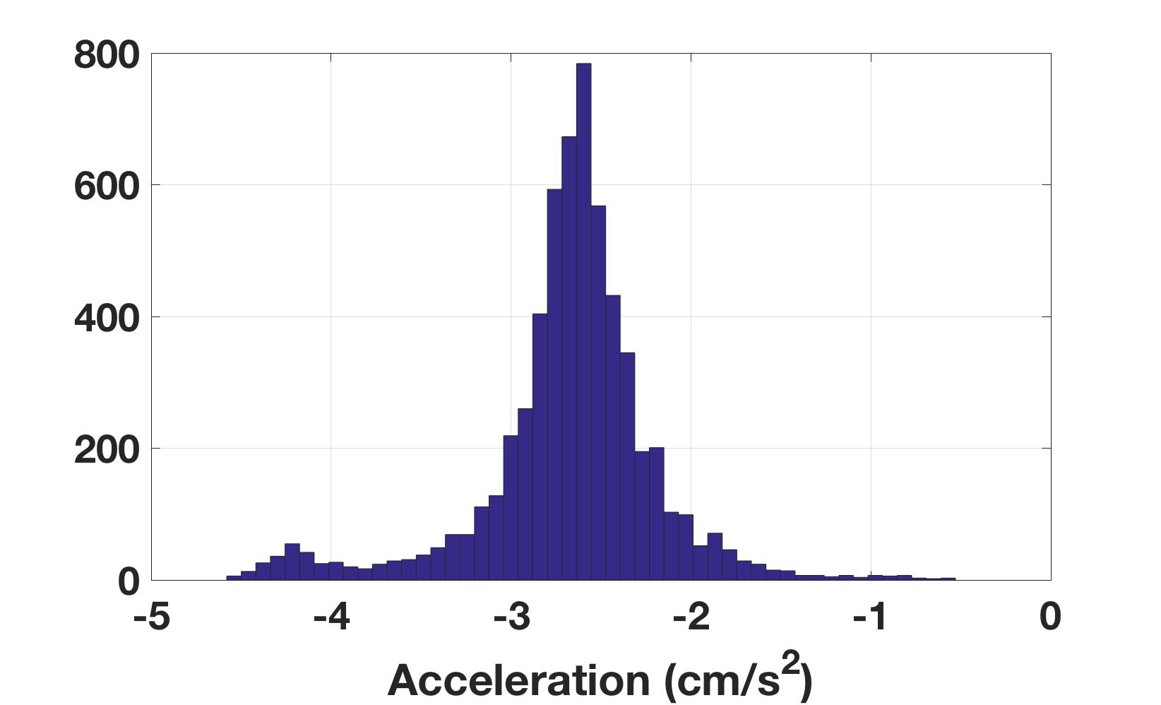
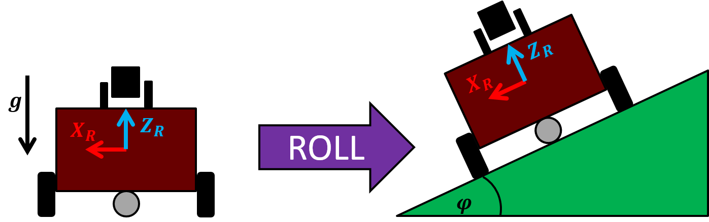
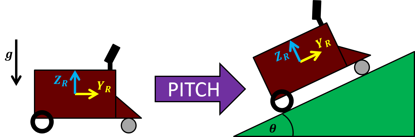
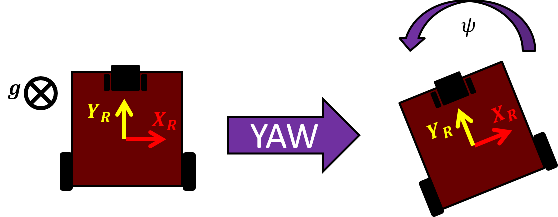
Figure 12: Cartoon of Pheeno at different orientations representing the roll, pitch, yaw convention.
Gyroscope Calibration
Gyroscopes typically don’t need much calibration. Again, an assumption about the sensor noise should be made. The gyroscope is assumed to have AGWN like the accelerometer. The analysis supporting this assumption is the same as provided in the Accelerometer Calibration section and will not be shown here. Calibrating a gyroscope only requires subtracting a resting bias. This involves simply averaging the gyroscope measurements in each direction when Pheeno is at rest on a level surface, then saving this information and subtracting the average from any reading.
It should be noted that the axis the gyroscope measures rotation about are the same as the accelerometer. This means any measurement made by the gyroscope should be transformed to Pheeno’s reference frame through the rotation matrix found in the Accelerometer Calibration section. It is up to the user whether to subtract an average of the transformed measurements from transformed measurements or subtract the average untransformed measurements from untransformed measurements then transforming the result. The latter is preferred but both are valid.
Magnetometer Calibration
Magnetometers are typically the sensor that requires the most frequent calibration. Like the accelerometer, the magnetometer measures a theoretically constant magnetic field vector with respect to the magnetometer’s orientation. However, these readings can easily be thrown off by large metal beams or wires with large electrical currents in buildings. For larger robots, the motors can cause throw off large magnetic anomalies, however, Pheeno uses very small low current motors so their effects can be ignored. In an ideal scenario, the magnetometer would just read the magnetic field of the earth, which is different depending on the user’s location around the globe. With that said, even if the magnetometer were calibrated at the factory it was produced in, those calibration values would be invalid other places. For this section, it will be assumed the magnetometer is only reading the Earth’s magnetic field. Ways to overcome or recognize anomalies in the magnetic field are possible but will not be covered.
The ideal response surface for a 3-axis magnetometer is a sphere centered at the origin. This means if the user rotates the magnetometer while taking readings, a well calibrated magnetometer will produce point readings on a sphere with a radius equal to the magnitude of the magnetic field present. Figure 13(a) shows uncalibrated data taken from the magnetometer on-board Pheeno. The data was taken at 1Hz increments while the sensor was slowly rotated about each axis. The plot is a various 2D slices from the 3D sphere to illustrate the fact that the slices are not centered at the origin and the response sensitivity is different along each axis (they are not equal radius circles). These are often referred to as hard iron and soft iron errors or biases, respectively.
Hard iron biases are typically the largest source of error and usually the easiest to account for. To correct this, record the maximum and minimum field measurements along each axis while rotating the magnetometer. Once the user is satisfied the magnetometer has taken sufficient measurements in each orientation, the average between the max and min magnetometer reading along each axis is equal to the hard iron bias in each direction.
To correct for the soft iron bias correctly, the response surface from the raw measurements of the magnetometer should be deconstructions into their elliptical principle axis to create a $3\times3$ correction matrix to transform the general ellipsoid to a sphere. This is pretty involved and more importantly can be approximated in a much easier way. An explanation of the mathematics behind the full calibration method can be found at [2].
A decent approximation for this process is to simply scale the response along each axis with the maximum and minimum measurements already calculated previously. First a scale factor, $s$, is calculated,
where,
This average scale factor is then projected onto each axis as a gain,
This approximation of the full calibration is a simple orthogonal rescaling; equivalent to a diagonal $3\times3$ calibration matrix.
The calibrated data is then found by subtracting the hard iron bias from the raw measurement in each axis and scaling the difference. For example the calibrated magnetometer reading, $\vec{M_{cal}}$, of a raw measurement, $\vec{M_{raw}} = [M_x \hspace{1mm} M_y \hspace{1mm} M_z]$, with hard iron bias vector $\vec{b_{HI}} = [b_x \hspace{1mm} b_y \hspace{1mm} b_z]$ and scaling matrix $\boldsymbol{G} = diag(sx,sy,sz)$ would be,
Figure 13(b) shows data taken after calibration. Compared to the uncalibrated data, the circles are now concentric and approximately circular.
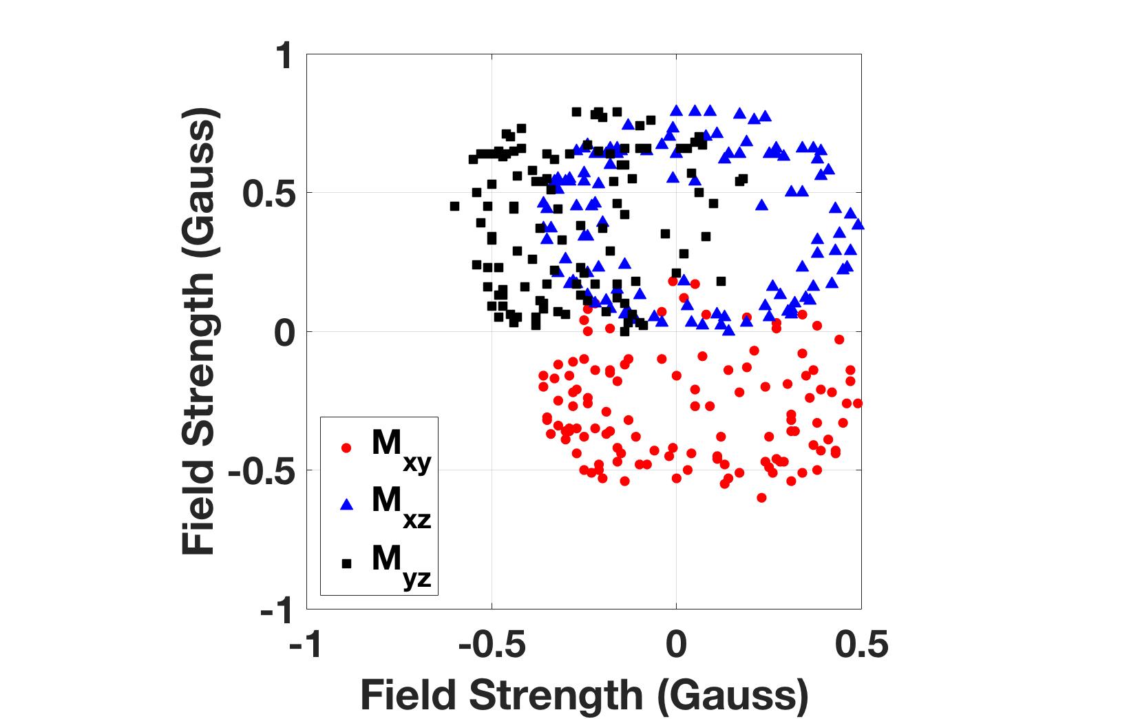
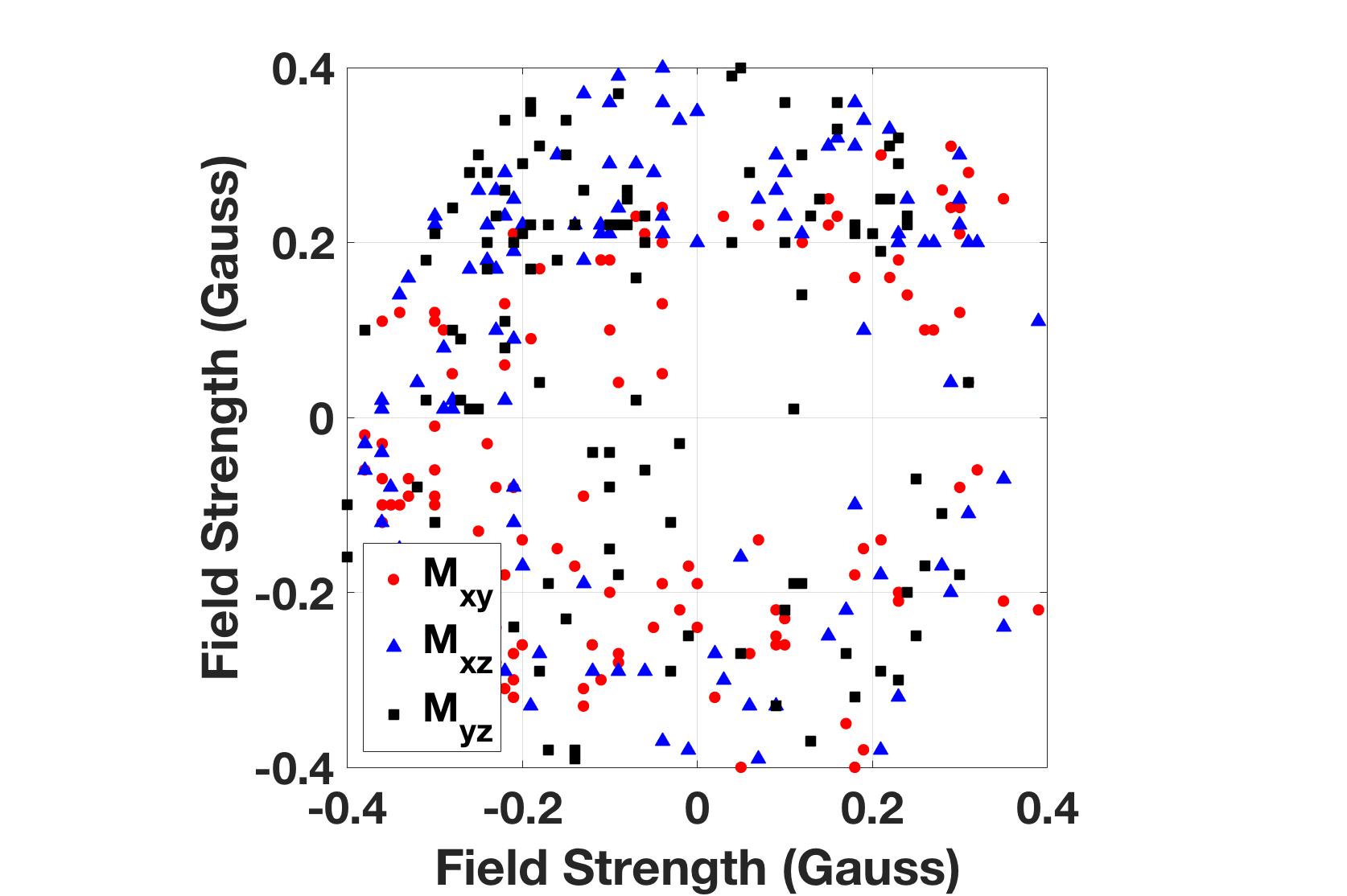
Figure 13: Several slices of the magnetometer measurements along the principle plains.
Motor Encoder Calibration
Motor encoders do not require any sort of calibration. However, the data (which is the number of counted rotations) has to be transformed to some usable units. For generality, the encoders will be assumed to count $n$ times per rotation of the extended back shaft and there will be a $g$ gear ratio from the measured extended back shaft to the wheel shaft. From this assumption, the numbers of radians the drive shaft has traveled per count, $x$, would be,
From this transformation, the linear distance a wheel would travel (assuming no slipping) and the rotational velocity of the wheel shaft can be calculated.
An important note that can cause some issues is these counts become very large very quickly. Usually these counts are stored in an integer variable on board your robot’s processor which only allows n-bit ranges ($2^{n}$). In Pheeno’s case signed integers are stored in a $16$-bit variable. This means signed integers can only be stored from $[-32768,32767]$ once this range is surpassed, the number will roll over. This means if the count were supposed to increment to $32768$ (outside the range) it would actually go to $-32768$. This can cause velocity and position estimates to go haywire if not expected. Standard conditional statements inside the robot’s code can alleviate this issue but users should still be aware of this issue.
Sensor Fusion for State Feedback
This section will go through complementary filters that are used on board Pheeno to fuse the sensor measurements to determine the robot’s state (position, velocity, orientation, etc.). It will also briefly go into using the sensors that sense the robot’s surroundings (IR distance sensors and camera) to determine reliable information about the environment.
The Complementary Filter (Basic) section will go over complementary filtering of sensors in a very basic sense with limited mathematics to give the user an intuition. The Complementary Filter (Advanced) section will introduce complementary filters in a more mathematically rigorous sense. The Complementary Filter Design for Pheeno section briefly describes the complementary filters used on board Pheeno.
Complementary Filter (Basic)
A complementary filter is an easy to implement sensor filter that joins two state estimates together. These estimates are required to be accurate on different time scales. Meaning that one must be able to capture fast and aggressive changes while the other maintains a consistent reading that will stay correct for long periods of time after the aggressive maneuver (the measurement does not drift). For example, to determine the robot’s orientation about one axis, gyroscope measurements can be combined with magnetometer or accelerometer measurements. The gyroscope is able to pick up quick motions well but after long periods of time will drift and its angle estimates will become wrong, while the accelerometer and magnetometer will determine the correct orientation when the motions are less aggressive.
Complementary filters are very similar to proportional, integral, derivative controllers in nature. They are easy and computationally inexpensive to implement on micro controller while still yielding extremely accurate measurements. Their major drawback is they may only fuse two measurements and do not give any intuition about how wrong their measurement estimates may be. The measurements are also required to have strengths in opposite frequency domains which is not always possible. Complementary filters are used on board Pheeno to estimate the robot’s roll, pitch, and yaw angle as well as body linear velocity estimates. For this small, relatively slow robotic platform, complementary filters are found to be just as effective as more advanced Kalman filters at a fraction of the computational expense.
These filters work by using high pass and low pass filters simultaneously. High pass filters allow high frequency signals while suppressing low frequency signals (such as drift of the gyroscope). Low pass filters act the opposite way by allowing low frequency signals while suppressing high frequency contents (like vibrational noise picked up by the accelerometer). In its most simple form, a first order complementary filter takes the form,
where, $m_{filter}$ is the filtered measurement, $m_{fast}$ is the measurement that is accurate over short timescales, $m_{slow}$ is the measurement that is accurate over long timescales, and $a \in (0, 1)$ is the filter gain that is to be chosen.
Choosing $a$ properly requires a bit of mathematics to fully understand but can be chosen and tweaked based on some intuition as well. Equation 3 can be looked at naively as an average. Two measurements are being averaged based on the users confidence in them during short time periods. The higher $a$ is chosen, the more the filtered measurement will rely on the fast measurement and will take longer to return to the slow measurement (which will be true when the aggressive maneuver has ended). The lower $a$ is chosen, the more the filtered measurement will rely on the slow measurement and will be more prone to short term noise. While this is not how these filters were formulated (the idea behind them was not averaging in this sense), it is good intuition to design these filters. The optimal choice for $a$ in a scenario will result in a filtered measurement that is able to capture very fast changes in the measurements as well as not have that measurement drift.
As a more concrete example, consider an accelerometer and gyroscope measurement being fused to determine a roll angle estimate. Using the first order complementary filter, the roll estimate at time $t$ after a time step of $\Delta t$ could be determined by,
This example essentially updates the new roll angle estimate, $rollAngle$, by combining $90\%$ of the gyroscopes update, $gyroRollRate$ with $10\%$ of the accelerometer’s update, $accRollAngle$. This combination will ensure the measurement won’t drift due to the accelerometer limiting the integration error and will still be accurate in short term estimates due to the majority of the updated estimate coming from the gyroscope.
Complementary Filter (Advanced)
While the basic complementary filter gives a basic understanding of the complementary filter, this section looks at it with slightly more mathematical rigor. Figure 14 shows an example block diagram of a complementary filter fusing a gyroscopic angle measurement with an accelerometer measurement. The gyroscopic measurement is integrated once to yield an angle then high pass filtered to avoid drift. The accelerometer measurement is low pass filtered to avoid the high frequency noise that plagues accelerometer measurements during fast rotations. When added these measurements complement each other’s weaknesses.

Using a first-order high pass and low pass filter, the transfer function in continuous time is,
:label: CFCont
where $T$ determines the cut-off frequencies. This now must be transformed to discrete time, as robots do not operate in continuous time. Using backwards difference, $s = \frac{1}{\Delta t}(1-z^{-1})$, in \autoref{eq:CFCont} leads to the final equation,
:label: CFGyroAcc
where, $\alpha = \frac{T}{T+\Delta t}$. Note, this is the same as Equation 3.
This still begs the question, how should the cut off frequency be chosen? The answer is an optimization problem which is beyond the scope of this paper and usually needs to be adjusted in application if the optimization is done. The filter needs to be designed such that there are constant amplification and small phase loss of all measurements. More specifically, this means setting the cut off frequency high enough such that the largest range of frequencies is measured by the accurate but noisy sensor with slow dynamics (accelerometer, magnetometer, etc.). This avoids the drift typical in faster sensors. When motions occur that are at higher frequencies than the dynamics of the slow sensor, the cut off frequency should be set low enough such that the expected phase loss of the slower sensor is compensated by the faster sensor (gyroscope, encoders, etc.).
It should be noted on a small slow robotic platform like Pheeno, it is possible to set only one cut off frequency and get reliable measurements. However, in faster more agile systems like quad rotors, more advanced techniques like a gain-scheduled complementary filter are required. This filter switches it cut off frequency or other design parameters depending on how aggressive a measured action is (acceleration measurements). There is also another representation of a second order complementary filter based on the Mahoney and Madgwick filter for more agile systems that can be used over a first order filter to capture more advanced dynamics [3, 4, 5].
Complementary Filter Design for Pheeno
Pheeno uses complementary filters to determine its orientation angles (roll, pitch, yaw) as well as its linear velocity. This involves fusing the robot’s sensors with slow dynamics accelerometer, magnetometer) with its fast drifting sensors (encoders, gyroscope). Using the same convention established in the Accelerometer Calibration section, the accelerometer’s measurements is combined with the gyroscopes measurements to determine roll and pitch angles of the robot. The magnetometer angular measurements are combined with the gyroscopic measurements to determine the yaw angle of the robot (heading). The accelerometer is combined with encoders to determine the robot body’s velocity.
This design mostly comes from experience working with the sensors and in application the best way to determine filter coefficients is to tune on a data set and gain intuition about the sensors from their data outputs. It is possible to model the sensor and determine these cut off frequencies in a more mathematically rigorous fashion but, when working with inexpensive robots with readily accessible parts, this method is faster with just as valid results.
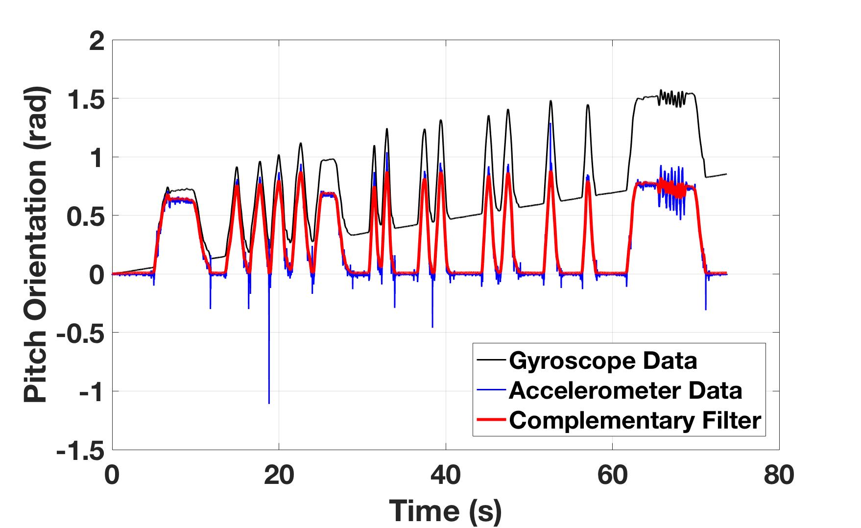
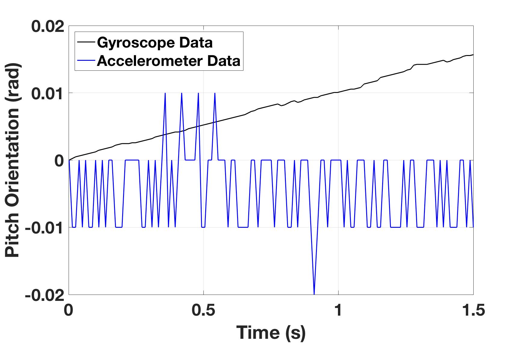
Figure 15: Orientation angle estimates from several sensors and a filtered combination while Pheeno was manually pitched about $45^{\circ}$ at different rates. (a) Accelerometer (blue), gyroscope (black), and complementary filter (red) estimate of Pheeno’s pitch angle. (b) A zoomed in section of (a).
Figure 15 shows the time evolution of the angular orientation estimate for Pheeno about its x-axis (pitch) as it was manually pitched from a level table to about $45^{\circ}$ over different periods. The filter take the form of \autoref{eq:CFGyroAcc}. To determine the parameter of the complementary filter equation, $\alpha = \frac{T}{T+\Delta t}$, refer to Figure 15(b). This data was sampled at $100$ Hz so $\Delta t = 0.01$. This leaves $T$, the time constant of the system. A rule of thumb used here is to determine the time when the fast sensor, in this case the gyroscope, drifts out of the error of the slow sensor, in this case the accelerometer, when the system is at rest and the slow sensor’s measurement is correct. For this case Figure 15(b) shows the gyroscope’s pitch estimate drifting outside the $0.01$ rad error envelope of the accelerometer after $1$ s. Plugging this into the equation for $\alpha$ yields, $\alpha = 0.99$. A similar process is done for each axis of rotation on the robot.
Further analysis of Figure 15 gives a good idea of how this fusion is performing. It is very apparent the pitch estimate from the gyroscope (black line) is drifting away from the true rotation range but is still capturing the rotation rate correctly especially during higher frequency rotations like between $t = 65$ s and $t = 70$ s. The accelerometer’s estimate (blue line) is not drifting but there are very apparent spikes when the robot makes contact with the table again and during the high frequency rotation between $t = 65$ s and $t = 70$ s. The complementary filter with $\alpha = 0.99$ captures the best of both of these sensors. There is no apparent spiking or noise from the accelerometer measurements and the estimate is not drifting.
References
[1] Eitel E. Basics of Rotary Encoders: Overview and New Technologies; 2014. Accessed: 2017-03-01. http://machinedesign.com/sensors/basics-rotary-encoders-overview-and-new-technologies-0.
[2] Ozyagcilar T. Calibrating an eCompass in the Presence of Hard- and Soft-Iron Interference; 2015. Accessed: 2017-03-01. https://www.nxp.com/files-static/sensors/doc/app_note/AN4246.pdf.
[3] Yoo TS, Hong SK, Yoon HM, Park S. Gain-scheduled complementary filter design for a MEMS based attitude and heading reference system. Sensors. 2011;11(4):3816–3830.
[4] Madgwick SOH, Harrison AJL, Vaidyanathan R. Estimation of IMU and MARG orientation using a gradient descent algorithm. In: 2011 IEEE International Conference on Rehabilita- tion Robotics; 2011. p. 1–7.
[5] Mahony R, Hamel T, Pflimlin JM. Nonlinear Complementary Filters on the Special Orthogonal Group. IEEE Transactions on Automatic Control. 2008 June;53(5):1203–1218.