Introduction

This document describes the controller design for the motors that drive Pheeno as well as the higher level controller that navigates the robot from one location to another. To create these controllers accurate models of the motors and robot are needed. The choice of models and fitting will be discussed in the Modeling the Motors and Modeling the Robot sections. The controller design sections will address which sensors are used to calculate the desired feedback but the details are discussed in the observer design document and thus, will not be talked about here.

The simplest possible models are used to design controllers for Pheeno. To understand this choice, refer to the passage from George Box’s 1978 paper,

Now it would be very remarkable if any system existing in the real world could be exactly represented by any simple model. However, cunningly chosen parsimonious models often do provide remarkably useful approximations. For example, the law $PV = RT$ relating pressure $P$, volume $V$ and temperature $T$ of an “ideal” gas via a constant R is not exactly true for any real gas, but it frequently provides a useful approximation and furthermore its structure is informative since it springs from a physical view of the behavior of gas molecules.

For such a model there is no need to ask the question “Is the model true?”. If “truth” is to be the “whole truth” the answer must be “No”. The only question of interest is “Is the model illuminating and useful?”

The better known section header of this passage is,

All models are wrong but some are useful.

There is a need for the model to capture the properties of the system that are useful without overparamertizing or overelaborating the model. Using more intricate models than are needed makes the controller design more complicated and, more importantly, over fits the data used to parameterize the system which can cause this model to describe a certain data set more than the system it is meant to represent. With the use of feedback control, even simple models that do not describe the system completely can be controlled in desirable fashion.

Modeling the Motors

The first and arguably most important step towards controlling the system is designing a fast controller for the motors. To do this an accurate model of the motors must be created. Typically, this would be done by parameterizing the standard second order transfer function for a direct current (DC) motor,

$$P(s) = \frac{\dot{\Theta}(s)}{E_a(s)} = \frac{K_T}{(Js+b)(Ls+R)+K_BK_T}.$$

where $K_T$ is the gain relating the armature current to armature torque, $K_B$ is the gain relating the rotational velocity of the rotor to the back EMF in the armature circuit, $J$ is the inertial of the rotor, $b$ is the viscous friction acting on the rotor, $L$ is the inductance in the armature circuit, and $R$ is the resistance in the armature circuit.

However, for micro-metal gear motors, like the ones used on Pheeno, $L « R$. This allows for the second order system to be approximated by a first order system by setting $L=0$ yielding,

$$P(s) \approx \frac{K_T}{R(Js+b)+K_BK_T} = \frac{K}{Ts + 1}$$

where,

$$K = \frac{K_T}{Rb+K_TK_B} \hspace{1cm} T = \frac{RJ}{Rb+K_TK_B}.$$

To fit these parameters, the motors will be black box modeled using MATLAB’s system identification toolbox [5]. Two motors attached to Pheeno were given step voltages and sinusoidal voltages of frequencies between $0.1$ and $50$ Hz. The max sinusoidal frequency was chosen following the Nyquist sampling criterion which states a signal may only be recreated if it is sampled twice as fast as its highest frequency component. The rotor rotational velocities were measured with its encoders at a rate of $100$ Hz. The input and output time plots are shown in Figure 1.

Figure 1: The voltage input (top) and rotor velocity output (bottom) signals for a DC motor.

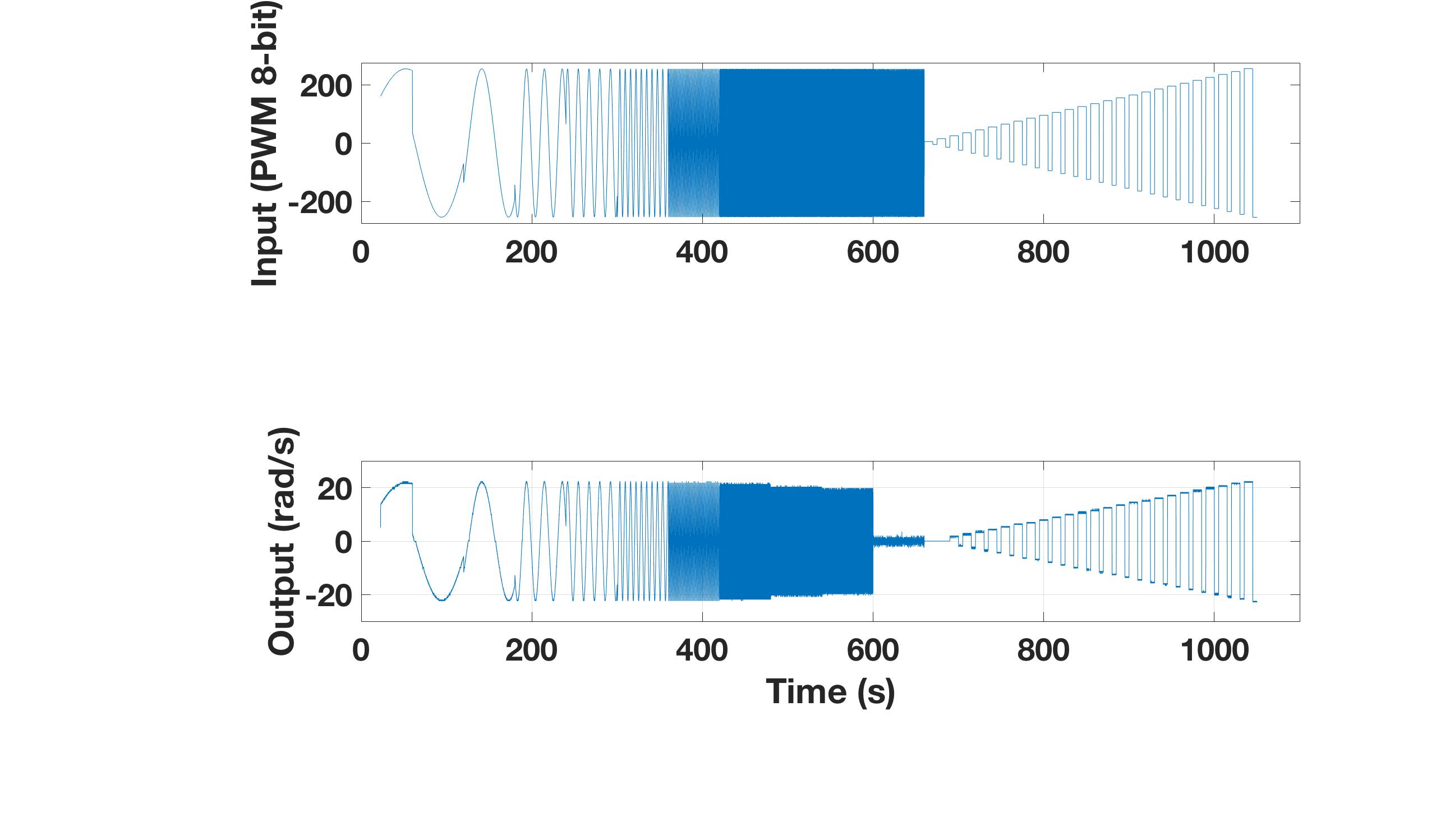
From these plots, it is apparent there is a large magnitude drop off as the frequency of the input signal increases. This is expected in a natural system like the DC motor.

This data is given to the system identification toolbox to fit a first and second order continuous model of the motor. As expected, the first and second order transfer functions yield equal “goodness of fit” to the data $\sim 80\%$. This fit is a little low but acceptable as a linear model is unable to represent nonlinear friction effects on the motor rotor. The first and second order system both have a pole at $\sim 36$ rad/s with the second order system also having a pole at $\sim 60,000$ rad/s. From this fitting it is obvious the dynamics of the motor are dominated by the single pole. The location of the pole fit also makes sense as the magnitude of the sinusoidal response begins to decay around $30$ rad/s as is expected with roll off caused by a pole.

This leaves the first order approximation of the system.

$$P(s) = \frac{2.9876}{s+36.07}$$

The model compared to a set of validation data can be seen in Figure 2.

(a)

(b)

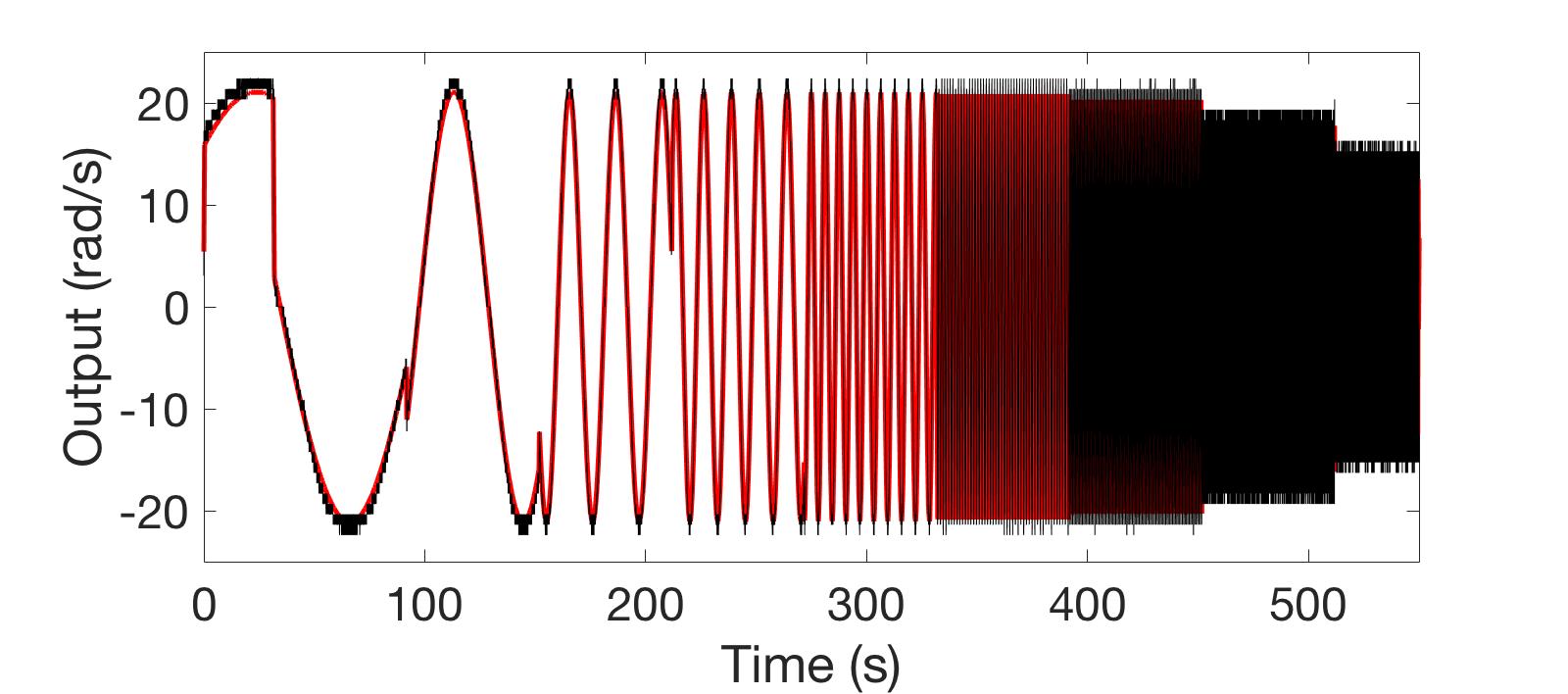
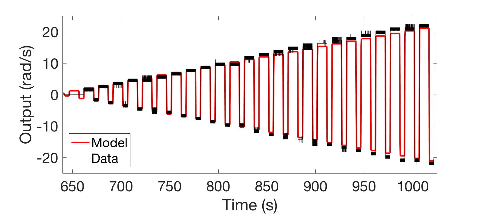
Figure 2: The first order DC motor model (red) compared to validation data (black)

Controlling the Motors

Continuous Consideration

From this plant it is possible to design a controller so that the motor responds in a desired way. For this application it is desirable to make the motors follow step commands (and rejects step disturbances) as fast as possible with no overshoot. From the internal model principle, a proportional integral (PI) controller is enough to satisfy these requirements.

Figure 3: A block diagram representation of a standard negative feedback loop.

This formulation leads to a standard feedback problem that must be solved. Figure 3 shows a block diagram of standard negative feedback loop with the symbols that will be used here. The plant, $P(s)=\frac{2.9876}{s+36.07}$, was found previously, a PI controller, $K=g\frac{s+a}{s}$, needs to be designed, and a pre-filter, $W=\frac{a}{s+a}$, needs to be incorporated to reduce the overshoot caused by the zero of the controller. Here, the sensor dynamics, $H$, are assumed to be ideal.

Typically, in a classroom setting, a pole placement method would be employed to match the nominal closed loop system to some desired closed loop system. In this case, a slightly different method will be employed. The plant here is a nominal representation of the system. This means there are higher order dynamics present in the system that are not modeled so the gain chosen cannot be very high and the dominant pole modeled here can be slightly or significantly off. First, $a$ will be chosen with these real world constraints in mind, then $g$ will be chosen such that there is no overshoot and the motors spin up as fast as possible.

First, notice the pre-filter is a stable low pass filter (presuming $a > 0$). This means it will create a natural delay on the reference signal depending on how small $a$ is chosen. Thus $a$ should be chosen to be large such that this delay does not significantly slow down the motor’s response to low frequency reference commands and does not restrict the magnitude of desired higher frequency signals. However, it should be chosen low enough that the integral term of the controller does not become too large and exacerbate the integral windup problem caused by motor saturation (which will be addressed later). Secondly, the proposed open loop system’s ($KP$) root locus will result in two different looking root locus depending on how $a$ is chosen. Figure 4 shows an example of both root locus. Note choosing $a$ larger than the dominant pole of the modeled motor has two critical damping points. The left critical damping point requires a much larger gain and thus will not be considered. The right critical point will shift left as $a$ is chosen closer to the pole of $P$ making the closed loop system’s response faster. To make the system as fast as possible, choose $a = 36.07$ so it cancels the pole of the motor. Typically, this is not a good idea because of modeling errors that cause this cancellation to not be true in reality. However, because it is a very stable pole, this choice does not have such severe consequences as model error will result in one of the two root locus represented in Figure 4.

(a)

(b)

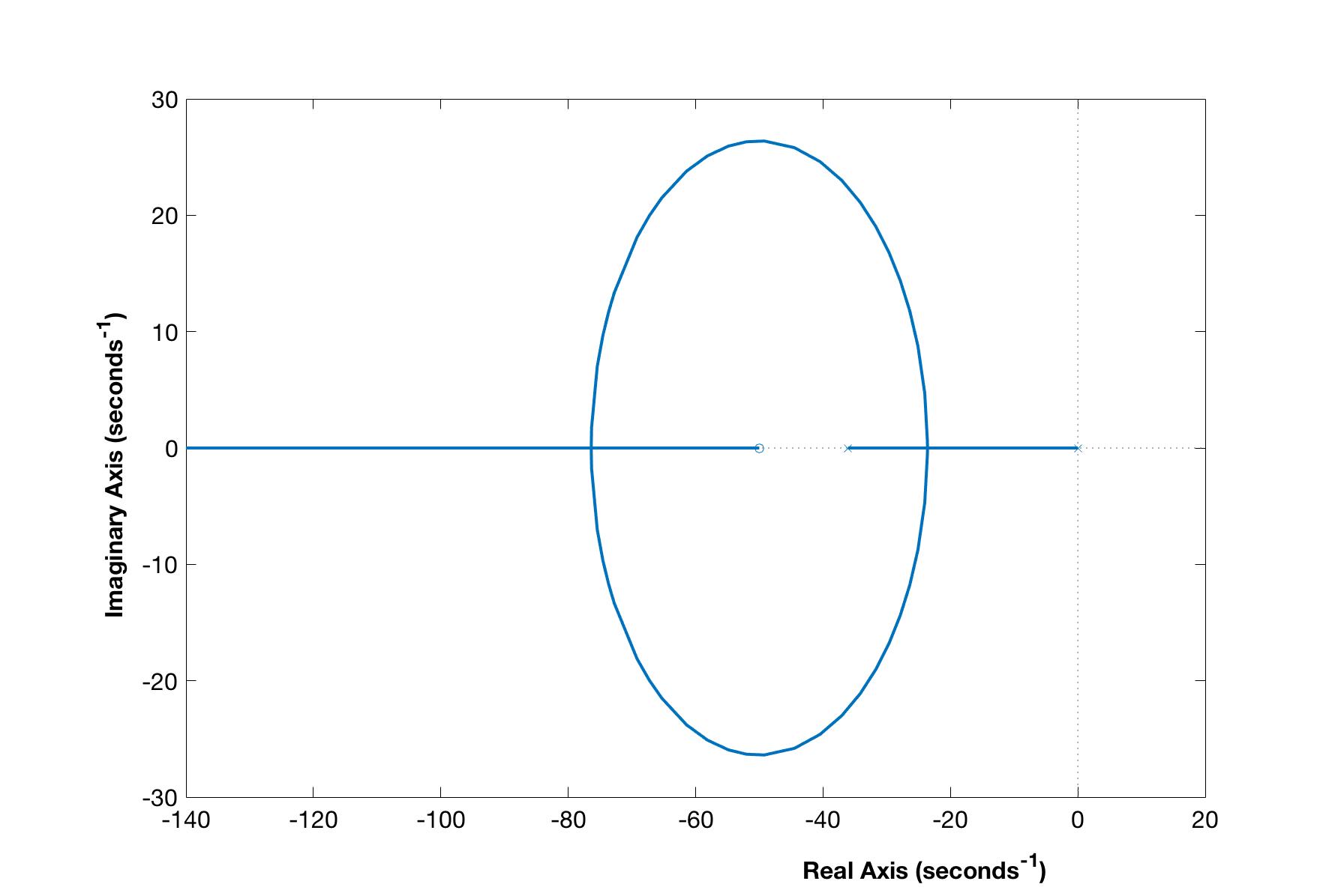
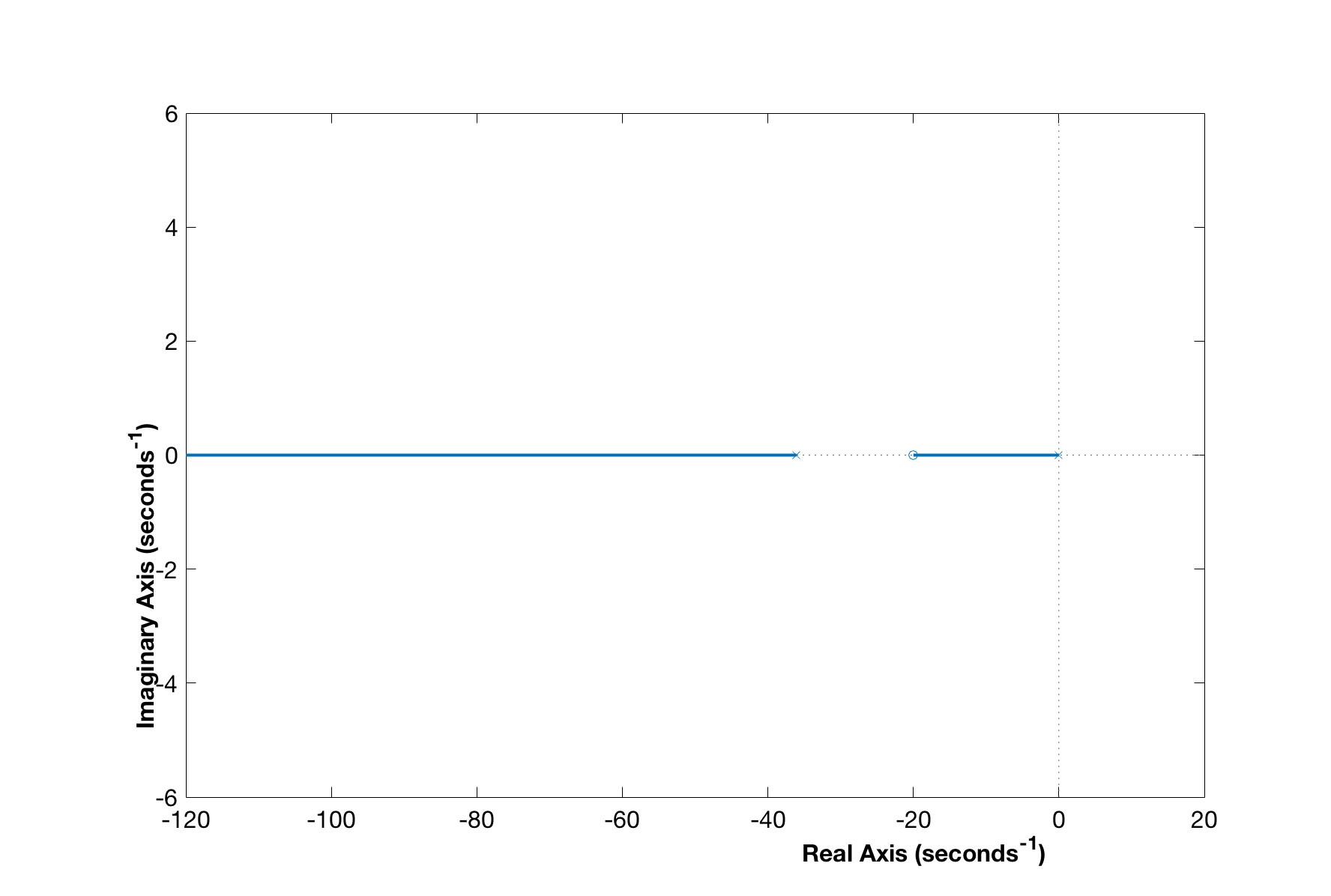
Figure 4: The root locus of Pheeno’s motors where the zero of the controller is chosen larger (top) and smaller (bottom) than the modeled pole of the motor.

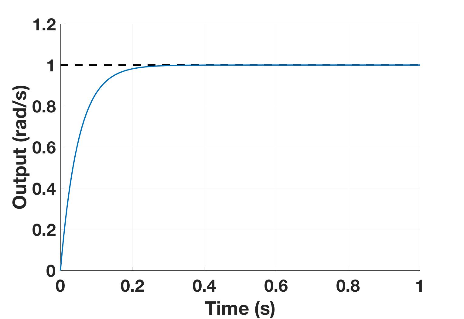
The gain, $g$, is chosen such that the rise time of the system is $<0.5$ s. Figure 5 shows a simulated step response of this controller and modeled plant which behaves as expected.

Figure 5: The simulated step response of the designed continuous motor control loop.

Dealing with Integral Windup

Integral windup is a problem that occurs in controllers containing integral terms when a large change in the reference command occurs. For example, if Pheeno is suddenly commanded to go from rest to full speed there will be a large error initially that will get smaller as Pheeno begins to reach its top speed. However, during this time the integral term of the controller will be compounding this error and cause an overshoot until enough error has occurred in the opposite direction to offset it. This gets worse when saturation of actuators are considered. In this case, a naive controller can require an output larger than what can be produced by the actuator. This causes integration error to continue to compile without knowledge that the error it is trying to rectify is beyond the capabilities of the system.

There are several ways to address this issue. In Pheeno, this issue is addressed by adding a secondary feedback loop that limits the integral term when motor saturation has occurred. Figure 6 shows this feedback loop in block diagram form. This feedback loop only kicks in if the controller’s desired output is higher or lower than the actuator can output. When saturation occurs, the feedback loop keeps the integral term from compounding when the error cannot be reduced. Typically the tracking gain, $K_t$, is chosen to be equal to the integral gain, $K_i$, but higher values can cause better performance [2].

Figure 6: Comparison of model to motor output for several reference commands.

Discrete Time Adaptation

It would be naive to just throw this controller onto the robot and assume the motors will respond as they were designed to. If the controller were designed in the continuous domain without accounting for the delays created by the sampling of the microcontroller, it is very likely the control would be unstable at worse or not exhibit the designed properties at best. The Teensy microcontroller can easily perform control loops at $100$ Hz. Thus a sampling time of $0.01$ is chosen to design the motor control around.

First, the plant should be transformed from the continuous domain to the discrete domain. There are many options to transform a continuous plant represented in the s-domain to the discrete time z-domain. For the plant, a zero-order hold (ZOH) conversion is chosen as that best represents the type of hold circuit that will be used in sampling the motor. The controller designed in the continuous case is transformed using the bilinear transformation to better approximate the continuous behavior of the controller in the discrete space.

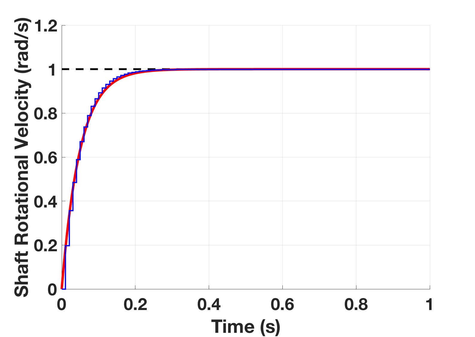
This control case is ideal as the sampling time is very fast compared to the desired rise time. Thus, the continuous system is very close to the discrete system. Figure 7 shows the step response of the discrete designed system with the continuous designed system. However, in general this will not be the case and the continuous system would need to be augmented with an additional gain to get the desired response characteristics or redesigned entirely.

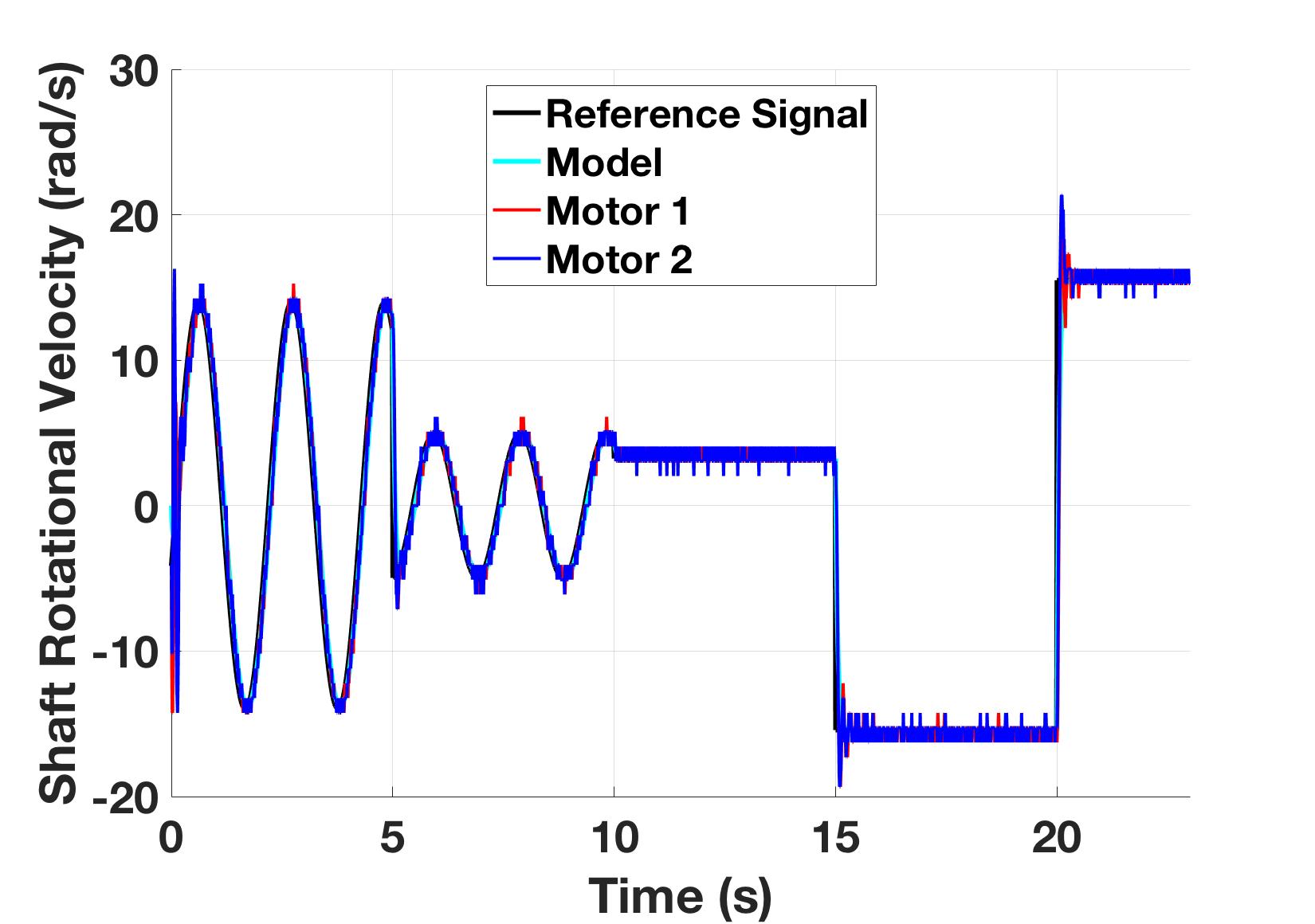
To validate this control, several known commands are given to two different motors on two different robots. The model’s prediction is compared to the motor outputs in Figure 8. For large jumps in the reference command, like the last two step commands, the integral windup overshoot is apparent but not overwhelming. This could be remedied with a less aggressive controller or putting a more restrictive low pass pre-filter on the reference commands. This would slow down the response considerably which is undesirable.

Figure 7: Comparison of simulated step response of the designed continuous and discrete motor control loop. The (blue) line shows the discrete time step response and the (red) line shows the continuous step response.

Figure 8: Comparison of model to motor output for several reference commands.

Modeling the Robot

Pheeno is by default a differential drive robot. This means each wheel can be controlled independently to produce desired motion. However, this makes the robot a coupled system resulting in a multi input multi output system which can be tricky to control properly. To simplify this, a decoupled kinematic model is used to represent Pheeno’s motion and control its position and orientation in a global reference frame. This can be done since Pheeno is so light and its motion is dominated by the motor torques. An extremely in depth analysis about when this assumption can be used is done by [1] in his master’s thesis.

Figure 9: Representation of Pheeno in a Cartesian coordinate frame.

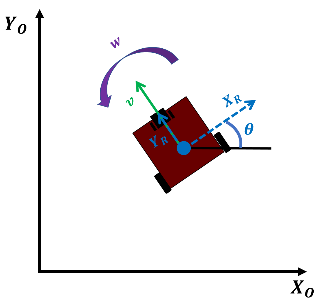
Consider Pheeno in an inertial reference frame ${X_o, Y_o}$ as shown in Figure 9. Pheeno’s basic motion model is, what is commonly referred to as, the unicycle model.

$$ \begin{bmatrix} \dot{x} \\ \dot{y} \\ \dot{\theta} \end{bmatrix} = \begin{bmatrix} \cos{\theta} & 0 \\ \sin{\theta} & 0 \\ 0 & 1 \end{bmatrix} \begin{bmatrix} v \\ w \end{bmatrix} $$

Eq. 1) The Unicycle Model

This model transforms the robot’s linear velocity, $v$ , and rotational velocity, $w$ , in Pheeno’s reference frame to velocity states in the inertial frame. However, the robot’s linear and rotational velocity cannot be controlled directly so another transformation is needed linking the rotational velocity of the wheels, $v_R$ and $v_L$ , to $v$ and $w$ . This relation is derived more thoroughly in [6].

$$ \begin{bmatrix} v_R \\ v_L \end{bmatrix} = \begin{bmatrix} \frac{1}{r} & \frac{L}{2r} \\ \frac{1}{r} & \frac{-L}{2r} \end{bmatrix} \begin{bmatrix} v \\ w \end{bmatrix} $$

Eq. 2) Unicycle Model Conversion

Here, $r$ is the wheel radius and $L$ is the axle length of the differential drive robot. Combining Equation 1 and Equation 2, yields the final relation between the wheel speeds of the robot and the velocity states in the inertial reference frame.

$$ \begin{bmatrix} \dot{x} \\ \dot{y} \\ \dot{\theta} \end{bmatrix} = \begin{bmatrix} \frac{r}{2}\cos{\theta} & \frac{r}{2}\cos{\theta} \\ \frac{r}{2}\sin{\theta} & \frac{r}{2}\sin{\theta} \\ \frac{r}{L} & \frac{-r}{L} \end{bmatrix} \begin{bmatrix} v_R \\ v_L \end{bmatrix} $$

Eq. 3) Individual Motor Unicycle Model

However, it is much more intuitive to use the unicycle model (Eq. 1) thus control will be done to create reference linear velocities, $v$ , and rotational velocities, $w$ , for the robot to follow. These will then be transformed to motor velocity commands using Equation 2.

In discrete time, this unicycle model takes the form,

$$ \begin{bmatrix} x \\ y \\ \theta \end{bmatrix}_{k+1} = \begin{bmatrix} 1 & 0 &0\\ 0 & 1 & 0 \\ 0 & 0 & 1 \end{bmatrix} \begin{bmatrix} x \\ y \\ \theta \end{bmatrix}_k + \begin{bmatrix} \Delta t \cos({\theta_k + \frac{\Delta\theta_k}{2}}) & 0 \\ \Delta t \sin({\theta_k + \frac{\Delta\theta_k}{2}}) & 0 \\ 0 & \Delta t \end{bmatrix} \begin{bmatrix} v \\ w \end{bmatrix} $$

Eq. 4) Discrete-time Unicycle Model

This unicycle model has slight changes to the orientation model that can be found in a paper by [4]. Using this model over the usual one showed vast improvements in dead reckoning navigation for Pheeno.

Controlling the Robot’s Motion

The approach to using the unicycle model to navigate Pheeno from an initial position to a goal position described here is using a layered architecture. This means using a high level planner to design way points for the robot to pass through, which are then translated to linear and rotational velocities of the robot, which are finally put through the fast PI controller of the motors. This section focuses on the middle component which decides the set points for the linear and rotational velocities.

Assume the high level planner has given an initial desired position $\vec{u} = [u_x \hspace{2mm} u_y \hspace{2mm} u_\theta]^T$ . From a Lyapunov stability analysis in [6] the controllers which produce stable global position tracking are,

$$v = K_p \rho \cos{\alpha}$$ $$w = K_p \sin{\alpha}\cos{\alpha} + K_\alpha \alpha$$

where $K_p > 0$ is a gain associated with radial distance error from the goal location, $\rho = \sqrt{(u_x - x)^2 + (u_y - y)^2}$ , and $K_\alpha > 0$ is a gain associated with the robot’s heading error from the goal orientation, $\alpha = atan2(\frac{u_y - y}{u_x - x})$ . It should be noted the heading error, $\alpha$ , is bounded $[-\pi, \pi]$ which limits how large $w$ can get. However, the radial distance error, $\rho$ , is unbounded. Thus, it is typical in application to either know the bounds of $\rho$ when designing $K_p$ as a constant or choosing $K_p$ to be of the form,

$$K_p =\frac{v_0(1-e^{-a\rho^2})}{\rho}$$

which limits the maximum linear velocity of the robot to a designed $v_0$ . When designing for any application, the gains should be chosen carefully to avoid wheel slip caused by high accelerations. The controllers should also operate slower than the rise time of the motor controller ($\sim 0.1$ s) so the motors have a chance to produce the desired linear and rotational velocities demanded by the higher order controller.

References

[1] Iman Anvari. Non-holonomic differential drive mobile robot control & design: Critical dynamics and coupling constraints, 2013.

[2] C Bohn and DP Atherton. A SIMULINK package for comparative studies of PID anti-windup strategies. In Computer-Aided Control System Design, 1994. Proceedings., IEEE/IFAC Joint Symposium on, pages 447–452. IEEE, 1994.

[3] George EP Box. Robustness in the strategy of scientific model building. Robustness in Statistics, 1:201–236, 1979.

[4] Evgeni Kiriy and Martin Buehler. Three-state extended kalman filter for mobile robot localization. McGill University., Montreal, Canada, Tech. Rep. TR-CIM, 5:23, 2002.

[5] Lennart Ljung. System Identification Toolbox (Trademark) , 2017. URL https://www.mathworks.com/help/pdf_doc/ident/ident.pdf. Accessed: 2017-03-07.

[6] Kumar Malu and Sandeep Jharna Majumdar. Kinematics, localization and control of differential drive mobile robot. Global Journal of Research in Engineering, 14(1), 2014.